Ubiquity of Biomedical Measurements
Working within evidence-based medicine
Decisions for the individual patient rest on objective numbers.
Evidence-based medicine is the environment we work in.
Research and trials are distilled into objective decision rules — thresholds that say when to act.
But an evidence-based threshold is inert without a number from this patient.
Evidence sets the threshold. Measurement supplies the number. Together they help with the decision.
So a clinician must deal with a stream of numbers — each compared against the evidence.
A clinical day is a stream of numbers
Wherever care happens, something is being measured.
| Emergency & triage |
Heart rate, blood pressure, SpO2, temperature, glucose |
| ICU monitoring |
ECG, arterial pressure, capnography (CO2), respiration |
| Diagnosis |
ECG, EEG, blood biochemistry, cell counts, structural and functional imaging |
| Surgery & anaesthesia |
Depth of anaesthesia, end-tidal CO2, oxygenation |
| Rehabilitation |
Gait analysis, joint range of motion, muscle force, movement quality |
Every number triggers a decision
Evidence-based thresholds, applied to the individual patient.
| SpO2 = 88% |
→ |
Start supplemental O2 & investigate |
| Core temperature = 35.0 °C |
→ |
Active warming |
| Blood glucose = 45 mg/dL |
→ |
Immediate glucose administration |
| Gait speed = 0.8 m/s |
→ |
Flag fall risk / frailty |
A wrong number can mean a wrong decision.
Sources: SpO2 — BTS oxygen guideline (O’Driscoll et al., Thorax 2017); temperature (Brown et al., NEJM 2012); glucose — ADA (Standards of Care 2026); gait speed (Studenski et al., JAMA 2011).
These map onto what we will focus on
The course is organised around how each kind of number is obtained.
We focus on four types of biomedical variables:
- Kinematics & kinetics — movement, force, complex movement quantity and quality measures
- Pressure, flow, volume — blood pressure, airway pressure, spirometry, cardiac output
- Thermal — body and core temperature
- Biopotentials — electrical potentials from bioelectric phenomena (ECG, EEG, EMG), and bioimpedance
The last module will not be on measurement but an important class of medical devices used to diagnose and treat different conditions:
- Electrical Stimulation — electrode–tissue interface for stimulation; monophasic vs biphasic stimulation; functional electrical stimulation (FES); TENS; cardiac pacing
Two questions behind every number
1. How is this quantity actually measured?
2. How do we know we can trust the number? Is it accurate? Precise?
This module takes on question 2 — what makes a measurement trustworthy. The rest of the course takes on question 1 — one measurement problem at a time.
What is measurement?
Turning a physical quantity into a number we can act on.
Measurement is the process of assigning numbers to physical, abstract, or logical characteristics of an entity by comparing them to a known standard.
\[\text{measurement} = \underbrace{\text{value}}_{\text{how many}} \times \underbrace{\text{unit}}_{\text{which standard}}\]
A measurement result carries:
- a value and a unit — 37.0 °C, 120 mmHg
- a scale tells us what operations are legitimate on the measurement (next)
- an uncertainty — how far we trust it (Section 5)
The number is the end of this process — the objective quantity clinical decisions rest on.
Scales of measurement
What are we allowed to do with these numbers.
| Nominal |
labels only; no order |
Blood type (A, B, AB, O) |
Only evaluate equalities. \(x_1 = x_2\) or \(x_1 \neq x_2\) |
| Ordinal |
ordered, gaps incomparable |
mRS (0–6); Pain (0–10) |
Only evaluate inequalities. \(x_1 > x_2\), \(y_1 = y_2\) |
| Interval |
equal gaps; no true zero |
Temperature in °C |
All arithmetic operations only on differences. \(x_2 - x_1\) |
| Ratio |
equal gaps and a true zero |
Force, pressure, flow, temperature in °K |
All arithmetic operations on the measurements directly. |
0°C does not mean “no temperature”; 0 N does mean “no force”. That is the interval/ratio distinction.
Physical measurands are almost all ratio (force, pressure, flow, current) or interval (°C). Clinical assessments are often ordinal (mRS, pain, MRC strength).
mRS — Modified Rankin Scale: a 7-point ordinal scale (0 = no symptoms; 6 = death) for post-stroke disability. van Swieten JC et al., Stroke 1988;19:604–7. · MRC — Medical Research Council muscle strength scale: 6-point ordinal scale (0 = no contraction; 5 = normal power). MRC, Aids to the Examination of the Peripheral Nervous System, HMSO 1981.
Quiz — name the scale
Match each measurement to its scale: nominal · ordinal · interval · ratio.
| Blood volume (\(m^3\)) |
Ratio |
| Grades in TnI (\(A+, A, B, C, D, E, F\)) |
Ordinal |
| Temperature (\(^{\circ}F\)) |
Interval |
| Gender (\(M, F\)) |
Nominal |
| Age of a person (\(years\)) |
Ratio |
| Heart rate (\(bpm\)) |
Ratio |
| HIV status (\(+ve, -ve\)) |
Nominal |
| RGB colors (\(\#FE0034\)) |
Nominal |
| Wavelength of light (\(m\)) |
Ratio |
| Time since stroke (\(days\)) |
Ratio |
Sensors and the Signal Chain Model
Physical systems: energy and state
Every physical system has two things associated with it:
- Energy — what drives its dynamic behaviour.
- State — what tells how the system will evolve with time.
States are what we are primarily interested in measuring: voltage, charge, position, velocity, temperature, …
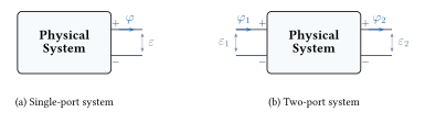
Information about a system’s states are available through its ports – interface through which energy, information (and possibly matter) is exchanged with the outside world.
![]()
Physical systems: energy and states are connected
A system’s total energy and its states are deeply connected.
Information about system’s memory
Memory comes from energy storage elements
The states of a system are our primary measurement interest (mostly).
Physical systems: energy and state
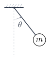
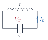
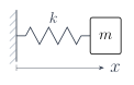
For an energetically closed system, its states can change even though its total energy remains the same:
Pendulum (State: \(\theta,\ \dot\theta\))
\(E = \tfrac{1}{2}m\ell^2\dot\theta^2 + mg\ell(1{-}\cos\theta)\)
LC circuit (State: \(V_C,\ I_L\))
\(E = \tfrac{1}{2}CV_C^2 + \tfrac{1}{2}LI_L^2\)
Mass–spring (State: \(x,\ \dot x\))
\(E = \tfrac{1}{2}m\dot x^2 + \tfrac{1}{2}kx^2\)
But for a system,
Total Energy changes \(\longrightarrow\) States change
Rule: System state measurement must not disturb the total energy of the system!
Connecting physical systems
One framework across every physical domain.
![]()
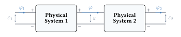
When we connect the ports of two systems together, the combined port assumes a single effort and a single flow.
These values are not free — they are set jointly by the physics of both systems: what each can supply, and what each will accept.
Consequence: neither system is left where it was before the connection.
Connecting physical systems
One framework across every physical domain.
![]()
Connecting two systems enables energy exchange.
The rate of energy transfer at the connection is determined by the common effort and flow variables:
\[ \text{power} = \frac{d E}{dt} = \text{effort} \times \text{flow} = \varepsilon \times \varphi \]
Consequence: whenever \(\varepsilon \times \varphi \neq 0\) at a port, energy flows and the system’s states change.
Connecting physical systems
One framework across every physical domain.
![]()
What are these effort and flow variables in different physical systems?
| Electrical |
voltage (\(v\)) |
current (\(\dot{q}\)) |
Mechanical
(translation) |
force (\(f\)) |
velocity (\(\dot{x}\)) |
Mechanical
(rotation) |
torque (\(\tau\)) |
angular velocity (\(\dot{\theta}\)) |
| Fluid |
pressure (\(p\)) |
volume flow rate (\(\dot{v}\)) |
| Thermal |
temperature (\(T\)) |
heat-flow rate \(\dot{q}\) |
(Thermal is the loose one — temperature × heat-flow is not literally power.)
Connecting physical systems — a worked case
A voltage source and a resistor.
Seperately, each sits at its own free condition:
| Voltage source |
\(V_s\) |
\(0\) |
| Resistor |
\(0\) |
\(0\) |
Each carries its own constraint — its physics, regardless of what it is attached to:
- Voltage source: \(\;V = V_s\;\) — the current can be anything
- Resistor: \(\;V = IR\;\) — neither variable is fixed on its own
When we connect the two systems, the port must satisfy both constraints at once: \[ \Longrightarrow \qquad \varepsilon = V_s, \qquad \varphi = \frac{V_s}{R} \]
What would happen if had a current source and a resistor?
\[ \Longrightarrow \qquad \varepsilon = I_s R, \qquad \varphi = I_s \]
Transducers, sensors, and actuators
The front door of every measurement.
- A transducer converts energy from one form to another.
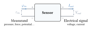
- A sensor converts a measurand into an (electrical) signal.
- An actuator converts an input energy or control signal into a controlled physical action — motion, force, or flow — that acts on a system.
The electrical signal carries information about the measurand.
\[ \text{Electircal Signal} = \mathcal{F}\left( \text{Measurand} \right) \]
Sensor signal chain
The spine of this whole course.
![]()
- Effort \(\varepsilon_m\) / flow \(\varphi_m\) from the signal source (human) contains information about the measurand of interest.
- Effort \(V_s\) / flow \(I_s\) is the sensor output that is related to the measurand.
\[ V_s = \mathcal{F}\left( \varepsilon_m \right) \]
\(\mathcal{F}\) represents the physics of the sensor relating the measurand to its output voltage/current.
Sensor signal chain when the source must be probed
Not every source emits the signal on its own.
Usually the source emits the signal, and we transduce it directly. (ECG, body temperature.)
Sometimes we must probe the system — apply a known energy and transduce its response.
![]()
Examples: Ultrasound (echo), bioimpedance (inject current, read voltage), pulse oximetry, imaging — structural measurements often work this way.
Loading – all sensors disturb measurands
Loading happens when physical system are connected together
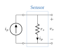
Consider a sensor whose resistance \(R_s\) changes in response to compressive force \(f_m \geq 0\) applied on the sensor, with the following physics,
\[ R_s = \mathcal{F}\left( f_m \right) = 10 + 0.5 \cdot \sqrt{f_m} \,\,\, \Omega , \quad f_m \geq 0 \]
Loading – all sensors distrub measurands
Loading happens when physical system are connected together
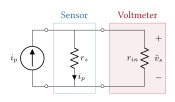
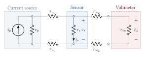
We connect a real voltmeter (input resistance \(r_{in}\)) to measure the voltage across the resister \(r_s\)
![]()
What is \(\hat{v}_s\)? \[\hat{v}_s = i_p \cdot \left( r_s || r_{in}\right) = v_s \cdot \frac{r_{in}}{r_s + r_{in}}\]
Loading — a realistic circuit
Real current sources, real wires, real voltmeters.
Assignment 1.1 — Real sensors have non-ideal sources and wires. Derive \(\hat{v}_s\) for the realistic circuit (finite \(r_p\), \(r_{w_1}\), \(r_{w_2}\), \(r_{in}\)). Understand the effect of the different resistances, and under what conditions (\(r_{w*}\) and \(r_{in}\)) is there no loading.
![]()
We have similiar loading effects in other domains as well (e.g. mechanical, thermal, egc.). \(\implies\) We should be careful when connecting physical systems.
Measurements from a real sensor
General input–output model.
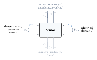
- \(x_m\): measurand of interest.
- \(x_i\): “Known” interferring / modifying inputs.
- \(e_n\): Unknown, random noise.
Each of these components will have an influence on the sesnor output \(y\), which can be represented as the following,
The general sensor output \(y\) is given by, \[ y = \mathcal{F}_m\left( x_m \right) + \mathcal{F}_i\left( x_i \right) + e_n\]
Sensor design tries to maximize \(\frac{\partial f}{\partial x_m}\), and minimize the \(\frac{\partial f}{\partial x_i}\) and \(e_n\).
All sensors are non-linear dynamical systems
Every sensor has dynamics — output lags, overshoots, or distorts fast inputs.
All sensors are non-linear, dynamical systems.
All sensors are non-linear dynamical systems
Every sensor has dynamics — output lags, overshoots, or distorts fast inputs.
General sensor behavior or characteristics can be divided into categories:
- Static characteristics - Response to constant inputs.
- Dynamic characteristics - Response to time varyng inputs.
- Noise characteristics - Response uncertainity associated for a given input.
The knowledge of these three characteristics will inform whether these sensor is suitable for an application.
Knowledge of the full functional form would provide complete characterization of the static and dynamic characteristics: \[ y(t) = \mathcal{F}_m\left( x_m(t) \right) + \mathcal{F}_i\left( x_i(t) \right) + e_n\]
We will need to identify these functions (at least \(\mathcal{F}\left(x_m\left(t\right)\right))\) in practice through a characterisation procedure.
Error Analysis in Measurements
Errors in Measurements
All measurements have errors
All measurements have error associated with them.
The appropriate interpretation of a measurement requires knowledge of the uncertainity associated with the measurement.
CODATA 2022
| Gravitational constant |
\(G\) |
\(6.674\,30 \times 10^{-11}\ \text{m}^3\text{kg}^{-1}\text{s}^{-2}\) |
\(1.5 \times 10^{-15}\ \text{m}^3\text{kg}^{-1}\text{s}^{-2}\) |
\(2.2 \times 10^{-5}\) |
| Proton mass |
\(m_p\) |
\(1.672\,621\,925\,95 \times 10^{-27}\ \text{kg}\) |
\(5.2 \times 10^{-37}\ \text{kg}\) |
\(3.1 \times 10^{-10}\) |
| Fine-structure constant |
\(\alpha\) |
\(7.297\,352\,5643 \times 10^{-3}\) |
\(1.1 \times 10^{-12}\) |
\(1.5 \times 10^{-10}\) |
| Rydberg constant |
\(R_\infty\) |
\(10{,}973{,}731.568\,157\ \text{m}^{-1}\) |
\(1.2 \times 10^{-5}\ \text{m}^{-1}\) |
\(1.1 \times 10^{-12}\) |
| Speed of light |
\(c\) |
\(299{,}792{,}458\ \text{m s}^{-1}\) |
exact |
exact |
| Planck constant |
\(h\) |
\(6.626\,070\,15 \times 10^{-34}\ \text{J s}\) |
exact |
exact |
| Boltzmann constant |
\(k_B\) |
\(1.380\,649 \times 10^{-23}\ \text{J K}^{-1}\) |
exact |
exact |
| Elementary charge |
\(e\) |
\(1.602\,176\,634 \times 10^{-19}\ \text{C}\) |
exact |
exact |
If all measurements have errors, how can we know some of them exactly?
Answer: Because those four are not measured — they are defined. In the SI, their numerical values are fixed by convention and the units derived from them: \(c\) defines the metre (1983), while \(h\), \(e\) and \(k_B\) define the kilogram, ampere and kelvin (2019 revision).
The uncertainty has not disappeared — it has moved. We no longer ask how well we know \(c\); we ask how well we can reproduce a metre in the lab.
Errors in Measurements
All measurements have errors
- What does \(G = 6.674\,30 \times 10^{-11}\ \pm 1.5 \times 10^{-15}\ \text{m}^3\text{kg}^{-1}\text{s}^{-2}\) mean?
- Reporting measurements as \(x \pm \Delta x\) are probabilistic statements \(\implies\) The true value of the parameter or measurements is likely to be in the range \(\left[ x - \Delta x, x + \Delta x\right]\) with some probability.
Errors in Measurements
All measurements have errors
Two important ideas are associated with measurements:
- Precision: Measure of the spread of a cluster of measurements for the same true value of the measurand.
- Accuracy: Measure of location of the spread of of measurements relative to the “true” value of the measurand.
Errors in Measurements
All measurements have errors
Accuracy and Precision naturally bring about two new concepts:
Random error: Contributes to the spread of the points — they tend to impact measurements both positively and negatively. \[ y_i = y_{true} + e_i \]
\(e_i\) is the random error; it is equally likely to be positive or negative.
Systematic error: Contributes to a consistent offset from the true value of the measurand. \[ y_i = y_{true} + y_{bias} \]
\(y_{bias}\) is the systematic error — a constant offset from the true value.
Overall, the total error in a measurement: \(y_i = y_{true} + y_{bias} + e_i\)
Random errors impair precision; systematic errors impair accuracy.
Random Errors in Measurements
Statistical Analysis of Random Errors
A commonly employed model for random errors in sensor measurements is the Gaussian or the Normal distribution.
\[ f\left( x \right) = \frac{1}{\sigma \sqrt{2 \pi}} \exp \left( {-\frac{1}{2} \left( \frac{x - \mu}{\sigma} \right)^2} \right) \]
Random Errors in Measurements
Statistical Analysis of Random Errors
\[ f\left( x \right) = \frac{1}{\sigma \sqrt{2 \pi}} \exp \left( {-\frac{1}{2} \left( \frac{x - \mu}{\sigma} \right)^2} \right) \]
Random Errors in Measurements
Statistical Analysis of Random Errors
\[ f\left( x \right) = \frac{1}{\sigma \sqrt{2 \pi}} \exp \left( {-\frac{1}{2} \left( \frac{x - \mu}{\sigma} \right)^2} \right) \]
Let \(\left[ x_1, x_2, \ldots, x_N \right]\) be a set of \(N\) independent measurements of the same measurand. The sample mean \(\hat{\mu}\) and sample standard deviation \(\hat{\sigma}\) are given by, \[ \hat{\mu} = \frac{1}{N} \sum_{i=1}^N x_i \quad \quad \hat{\sigma} = \sqrt{ \frac{1}{N-1} \sum_{i=1}^N (x_i - \hat{\mu})^2 } \]
These estimates allow us to quantify the mean and variance of the parent distribution of the measurand.
Note, that the sample mean \(\hat{\mu}\) and sample standard deviation \(\hat{\sigma}\) are themselves random variables, and will vary with each set of \(N\) measurements.
Random Errors in Measurements
Statistical Analysis of Random Errors
The estimates of \(\hat{\mu}\) and \(\hat{\sigma}\) are closer to the true values of \(\mu\) and \(\sigma\) as \(N\) increases.
Sampling distribution of the mean
The sample distribution of \(\hat{\mu}\) is also a Guassian distribution with the same mean \(\mu\) and a standard deviation of \(\frac{\sigma}{\sqrt{N}}\).
Random Errors in Measurements
Statistical Analysis of Random Errors
Sampling distribution of the mean
Precision of the sample mean \(\hat{\mu}\) increases with \(N\). This is called the standard error, \(\alpha\), \[ \alpha = \frac{\hat{\sigma}}{\sqrt{N}} \]
From \(N\) measurements, the true mean lies in the range \(\hat{\mu} - \alpha < \mu < \hat{\mu} + \alpha\) with probability \(\approx 68\%\).
Random Errors in Measurements
The error bar has its own error
Error in the Standard Error: \(\hat{\sigma}\) (and hence \(\alpha\)) is itself estimated from a finite sample — it too is a random variable. Its fractional error is,
\[\beta = \dfrac{1}{\sqrt{2(N-1)}} = \frac{\hat{\sigma} - \sigma}{\sigma}\]
- \(\beta\) depends only on \(N\) — not on \(\mu\) or \(\sigma\).
- The absolute uncertainty in \(\hat{\sigma}\) is \(\sigma\beta\).
- \(\hat{\sigma} \in [\sigma(1-\beta),\ \sigma(1+\beta)]\) with \(\approx 68\%\) probability.
- \(\beta\) falls slowly — as \(N^{-1/2}\).
Random Errors in Measurements
The error bar has its own error
The error in the error bar shrinks slowly.
Move \(\mu\), \(\sigma\) — the shape is unchanged. Only \(N\) narrows the \(\pm\beta\) band. Reaching \(\beta \approx 1\%\) (a trustworthy second significant figure in the error) needs \(N \approx 10{,}000\).
This discussion is imporant to decide how to report a measurements - how many digits are meaningful in the reported value and its error.
Reporting a measurement
Five repeat readings of grip force from a hand dynamometer (kg).
| 1 |
24.11 |
| 2 |
23.63 |
| 3 |
24.81 |
| 4 |
23.97 |
| 5 |
24.33 |
Compute, then report:
- sample mean \(\hat{\mu} = \frac{1}{N}\sum x_i\)
- sample SD \(\hat{\sigma} = \sqrt{\frac{1}{N-1}\sum (x_i-\hat{\mu})^2}\)
- standard error \(\alpha = \hat{\sigma}/\sqrt{N}\)
- error in the error \(\beta = 1/\sqrt{2(N-1)}\)
How would you write down the final result?
Reporting a measurement — work it through
Reporting grip strength measurements.
- \(\hat{\mu} = 120.85/5 = 24.17\) kg
- \(\hat{\sigma} = 0.4389\) kg, so \(\alpha = 0.4389/\sqrt{5} = 0.1963\) kg
- \(\beta = 1/\sqrt{8} = 0.354\) → the error itself is only good to \(\pm 35\%\)
- Uncertainty in the standard error is \(\beta \cdot \alpha = 0.354 \cdot 0.1963 = 0.0694\) kg → we are uncertain from the second significant digit onwards after the decimal place.
- So round \(\alpha\) to one significant figure: \(\alpha \approx 0.2\) kg
- Match the mean to the same decimal place: \(\hat{\mu} \to 24.2\) kg
- Report \(\;F = 24.2 \pm 0.2\) kg — not \(24.17 \pm 0.1963\) kg.
Discuss:
- Why is writing \(24.17 \pm 0.20\) kg a false claim?
- What would it take to earn that second digit?
Reporting a measurement — the awkward case
Six readings of a pressure sensor (mmHg). Compute \(\alpha\), then decide.
| 1 |
97.8 |
| 2 |
98.2 |
| 3 |
98.0 |
| 4 |
97.6 |
| 5 |
98.4 |
| 6 |
98.1 |
- \(\hat{\mu} = 98.017\)
- \(\hat{\sigma} = 0.286\), \(\alpha = 0.117\) mmHg
- One sig fig → \(\alpha \approx 0.1\): but that rounds \(0.117 \to 0.1\), a \(\sim 17\%\) shift in the stated error
- Exception: when the first significant figure of \(\alpha\) is 1, keep the second digit
- Report \(\;p = 98.02 \pm 0.12\) mmHg
- This rule ensures that the error due to round off is not too high.
Five golden rules (Source: Hughes & Hase, Measurements and their Uncertainties)
- The best estimate of a parameter is the mean.
- The error is the standard error in the mean.
- Round up the error to the appropriate number of significant figures (typically one significant digit).
- Match the number of decimal places in the mean to the standard error.
- Include units.
Propagation of Uncertainty
Raw measurements are seldom directly reported
Raw voltage, current measurements from sensors are seldom directly reported.
The raw measured quantities \(x\) are transformed through a mathematical formula to obtain the desired measurand \(y\).
If \(x\) has an uncertainty \(\Delta x\), what is the uncertainty in \(y\)?
- Does it depend on the function \(f(\cdot)\)? Yes
- Does it depend on \(\Delta x\)? Yes
Let the measured value of \(x\) be \(\overline{x}\) with uncertainty \(\Delta x\), thus the measur will be,
\[ \begin{split} y &= f(\overline{x}) \\ y + \Delta y &= f(\overline{x} + \Delta x) \end{split} \implies \Delta y = f(\overline{x} + \Delta x) - f(\overline{x}) \]
Propagation of Uncertainty
For small \(\Delta x\), we can linearize \(f(\cdot)\) about \(\overline{x}\) to obtain the uncertainty in \(y\),
\[ \Delta y \approx \Big\vert \frac{df}{dx} \Big\vert \cdot \Delta x\]
Propagation of Uncertainty
Propagation through Multivariable functions
We often compute parameters of interest using multiple raw measurements, each with its own uncertainty. Let the measurand \(y\) be a function of \(n\) measured quantities \(x_1, x_2, \ldots, x_n\), each with uncertainty \(\Delta x_i\),
\[ y = f\left( x_1, x_2, \ldots, x_n \right) \]
The uncertainty in \(y\) is given by the root-sum-square of the individual uncertainties,
\[ \Delta y = \sqrt{ \sum_{i=1}^n \left( \frac{\partial f}{\partial x_i} \Delta x_i \right)^2 } \]
Assumption: The uncertainties in \(x_i\) are mutually independent. If they are correlated, we need to account for them through the covariance terms.
Propagation of Uncertainty
Worked example — centre of pressure on a balance board
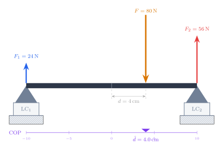
Two load cells read \(F_1, F_2\); the centre of pressure is
\[ F = F_1 + F_2 \quad \quad d = \frac{L}{2}\cdot\frac{F_2 - F_1}{F_1 + F_2} \]
Given the uncertainty in \(F_1\) and \(F_2\), what is the uncertainty in \(F\) and \(d\)?
\[ \Delta F = \sqrt{ (\Delta F_1)^2 + (\Delta F_2)^2 } \]
Uncertainty in \(F\) increases monotonically with that of \(F_1, F_2\).
The COP \(d\) is a more interesting case.
\[ \Delta d = \sqrt{ \left( \frac{\partial d}{\partial F_1} \Delta F_1 \right)^2 + \left( \frac{\partial d}{\partial F_2} \Delta F_2 \right)^2 } = \frac{2 L}{(F_1 + F_2)^2} \sqrt{ F_2^2\,(\Delta F_1)^2 + F_1^2\,(\Delta F_2)^2 } \]
For fixed reading error \(\Delta F_i\), \(\Delta d \propto 1/(F_1+F_2)^2\) — as the total load shrinks, the error in \(d\) blows up.
Propagation of Uncertainty
Watch the COP error grow as the total load drops
Static characterization
Response of a sensor to fixed inputs measurands
When performing static calibration, we must ensure that the sensor’s transient die out before reading the sensor output \(y_i\) for the input \(x_{m_i}\).
Static characterization
Response of a sensor to fixed inputs measurands
Static Calibration Data
Calibration data
| \(x_1\) |
\(y_1\) |
| \(x_2\) |
\(y_2\) |
| \(x_3\) |
\(y_3\) |
| \(\vdots\) |
\(\vdots\) |
| \(x_N\) |
\(y_N\) |
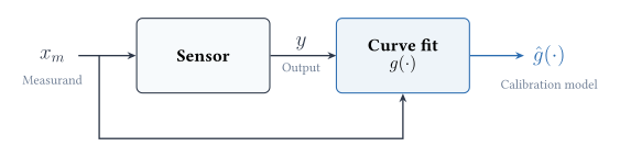
We fit this data to a function \(g(x_m)\) to build the static input-output model of the sensor.
\[ \hat{g}\left(x_m\right) = \arg \min_{g\left(x_m\right)} \Vert y - g\left( x \right)\Vert_2^2\]
We usually employ a least squares fitting procedure to identify the function \(g(x_m)\) or its parameters.
Polynomial models can generally be employed for capturing smooth non-linearities. \[ g(x) = \sum_{i=0}^m \beta_i \cdot x^i \]
Static characterization — calibration model
Fit a model to the calibration data to obtain \(\hat{g}(\cdot)\), then inspect the residuals.
We define the mismatch between measured value and the model prediction as the residual \(r\),
\[ r_j = y_j - \hat{g}\left(x_{m_j}\right) \]
Static characterization — calibration model
Using the static calibration fucntion \(\hat{g}\left(\cdot\right)\)
Once the function \(\hat{g}\left(\cdot\right)\) is esitmated, we can use it to estimate the measurand from the measurement: \(\hat{x}_m = \hat{g}^{-1}\left(y\right)\)
Static characterization — calibration model
Some sensors have hysteresis, making it difficult to use them.
Some sensors have hysteresis, which is the difference in measurements for the exact same input measurand, depending on whether the input is increasing or decreasing.
Dynamic characterization — calibration model
Identifying the dynamic characteristics of the sensor
Clinical motivation: A sidestream capnograph designed for adults has a long sampling tube and large analyser chamber — together these create a large time constant τ. A neonate breathes at 50–60 breaths/min (one breath every ~1 s). If an adult sampling line is used, the CO₂ waveform is smeared beyond recognition and ETCO₂ reads near zero — not because the sensor is broken, but because its dynamics are too slow for the signal. (numbers to be updated after reading the papers)
Static characteristics:
- sufficient for constant or very slowly varying measurands.
- insufficient for time-varying measurands.
When the measurand varies with time, the sensor dynamics cannot be ignored!
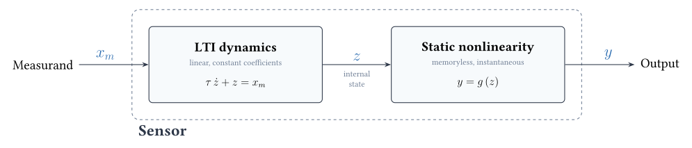
In general, sensor dynamics can be represented as a nonlinear differential equation.
For a linear time invariant (LTI) sensor, the differential equation becomes a linear constant coefficient one.
Dynamic characterization — calibration model
Identifying the dynamic characteristics of the sensor
![]()
The capnographic sensor difference understanding using the above model
Dynamic characterization — calibration model
Identifying the dynamic characteristics of the sensor
Dynamic characterization — calibration model
Identifying the dynamic characteristics of the sensor
![]()
Bandwidth of the signal is commonly used to capture the idea of how quickly a signal varies.
\[\text{Higher Bandwidth} \iff \text{Faster signal variation}\]
Bandwidth of the sensor tells the fastest signal that the sensor can track.
\[\text{Higher Bandwidth} \iff \text{Tracks faster signal variation}\]
For measuring time varying measurands, we must ensure: \[\text{Sensor Bandwidth} > \text{Signal bandwidth}\]
Dynamic characterization — calibration model
Identifying the dynamic characteristics of the sensor
Capnograph example: If we know \(\tau\), we can verify that the sensor’s bandwidth exceeds the signal’s bandwidth — and choose or reject equipment accordingly.
For LTI sensors, there are several ways dynamic characterization can be done. All these methods follow the same common template:
- Applying a characteristic test input signal \(x_m\left(t\right)\). (Example: impulse signal, step signal, sinusoids of different frequencies (chirp), white noise, etc.)
- Record the sensor’s response \(y\left(t\right)\)
- Estimate dynamic parameters, which contain information about the sensor’s bandwidth. (Parameter estimation, spectral estimation, etc.)
Dynamic characterization is more involved than static calibration.
Dynamic characterization of non-linear systems is more difficult than for LTI sensors, and we will need to make assumptions about the functional form of the non-linearities.