Consider an $p$-order stationary autoregressive model driven by white noise.
\[x_n = \sum_{k=1}^{p} a_kx_{n-k} + \epsilon_n\]where, $\epsilon_n$ is Gaussian white noise with zero mean and variance $\sigma_{\epsilon}^2$.
Let us assume that we have $N+$ sample of this AR process and we are interested in estimating the parameter $a_k$. We can arrange the data into a set of $M=N+1-p$ linear equations,
\[\begin{bmatrix} x_{0} & x_{1} & \cdots & x_{p-1} \\ x_{1} & x_{2} & \cdots & x_{p} \\ x_{2} & x_{3} & \cdots & x_{p+1} \\ % x_{p+1} & x_{p} & \cdots & x_{2} \\ \vdots & \vdots & \ddots & \vdots \\ x_{N-p} & x_{N-p+1} & \cdots & x_{N-1} \end{bmatrix} \begin{bmatrix} a_p \\ a_{p-1} \\ \vdots \\ a_1 \end{bmatrix} = \begin{bmatrix} x_{p}\\ x_{p+1}\\ x_{p+2}\\ \vdots\\ x_{N} \end{bmatrix}\] \[\begin{bmatrix} \mathbf{x}_{N-p, M} & \mathbf{x}_{N-p+1, M} & \cdots & \mathbf{x}_{N-1, M} \end{bmatrix} \mathbf{a} = \mathbf{x}_{N, M}\] \[\mathbf{X}_{N, M}\mathbf{a} = \mathbf{x}_{N, M}\]where, \(\mathbf{x}_{k, M}\) is a column vector whose elements are the past \(M\) of \(x_n\) starting from the instant \(k\); \(x_{k-M+1}\), \(x_{k}\) are the first and last elements of the vector, respectively. \(\mathbf{X}_{N, M}\) consists of the columns \(\mathbf{x}_{N-p, M}, \,\mathbf{x}_{N-p+1, M}, \, \ldots \, , \mathbf{x}_{N-p, M}\).
The least-squares estimate of $\mathbf{a}$ is given by,
\[\hat{\mathbf{a}} = \left(\mathbf{X}_{N, M}^T\mathbf{X}_{N, M}\right)^{-1}\mathbf{X}_{N, M}^T\mathbf{x}_{N, M}\]Post-multiplying \(\mathbf{x}_{N, M}\) by the pseudo-inverse will provide the least square estimate of \(\mathbf{a}\).
A simple example: Let us start with the simplest possible example of a AR process where \(p=1\).
\[x_n = a_1 x_{n-1} + \epsilon_n\]Lets assume that we have \(N\) samples of \(x_n\), we can then estimate the parameter \(a_1\) using the following,
\[\hat{a}_1 = \frac{\mathbf{x}_{N-1, M}^T\mathbf{x}_{N, M}}{\mathbf{x}_{N, M}^T\mathbf{x}_{N, M}}\]Running estimate of a AR process of order 1
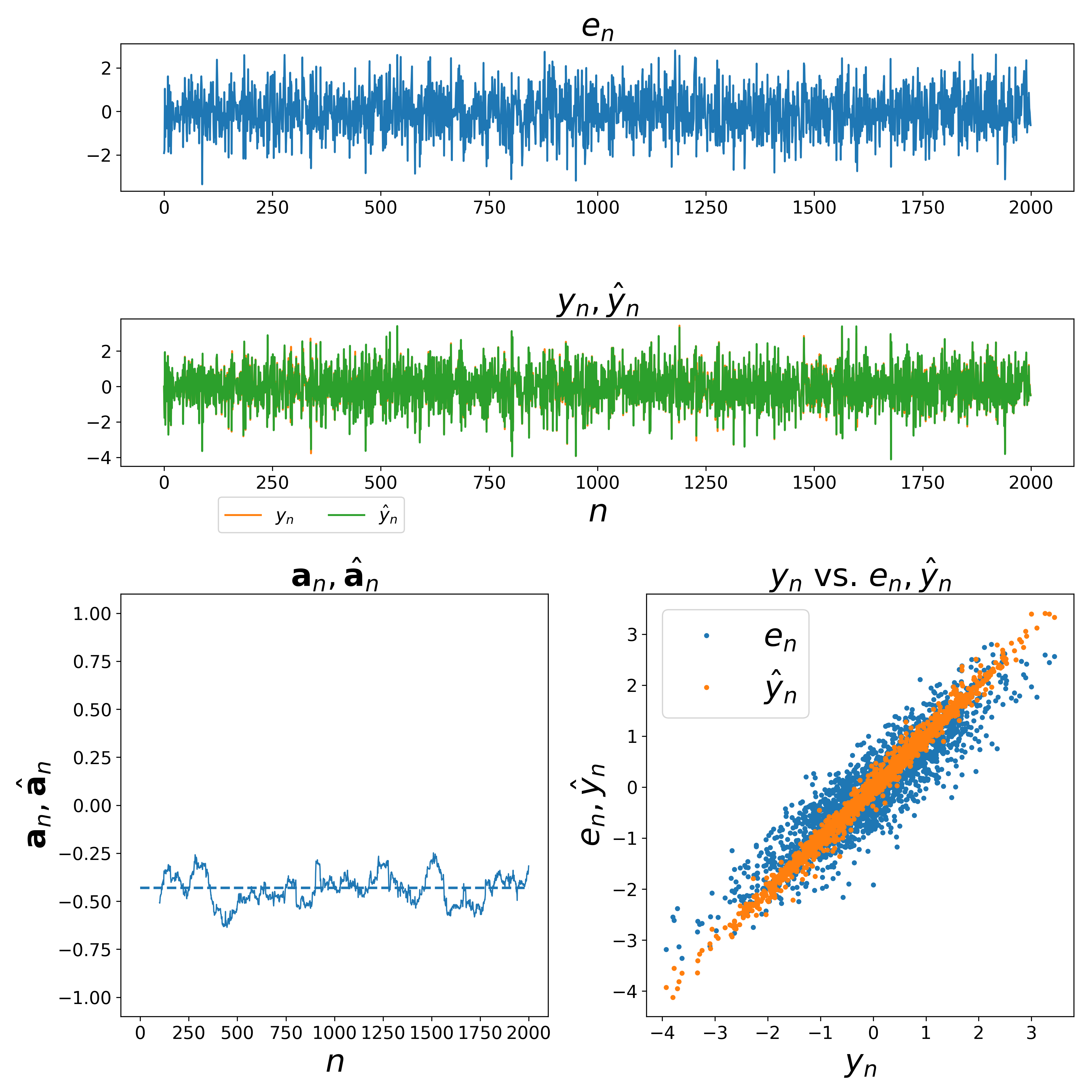
The following figure shows the result from an estimation procedure for a autoregressive process of order 1. The code used for generate this plot can be found here.
Running estimate of a AR process of order ‘p’
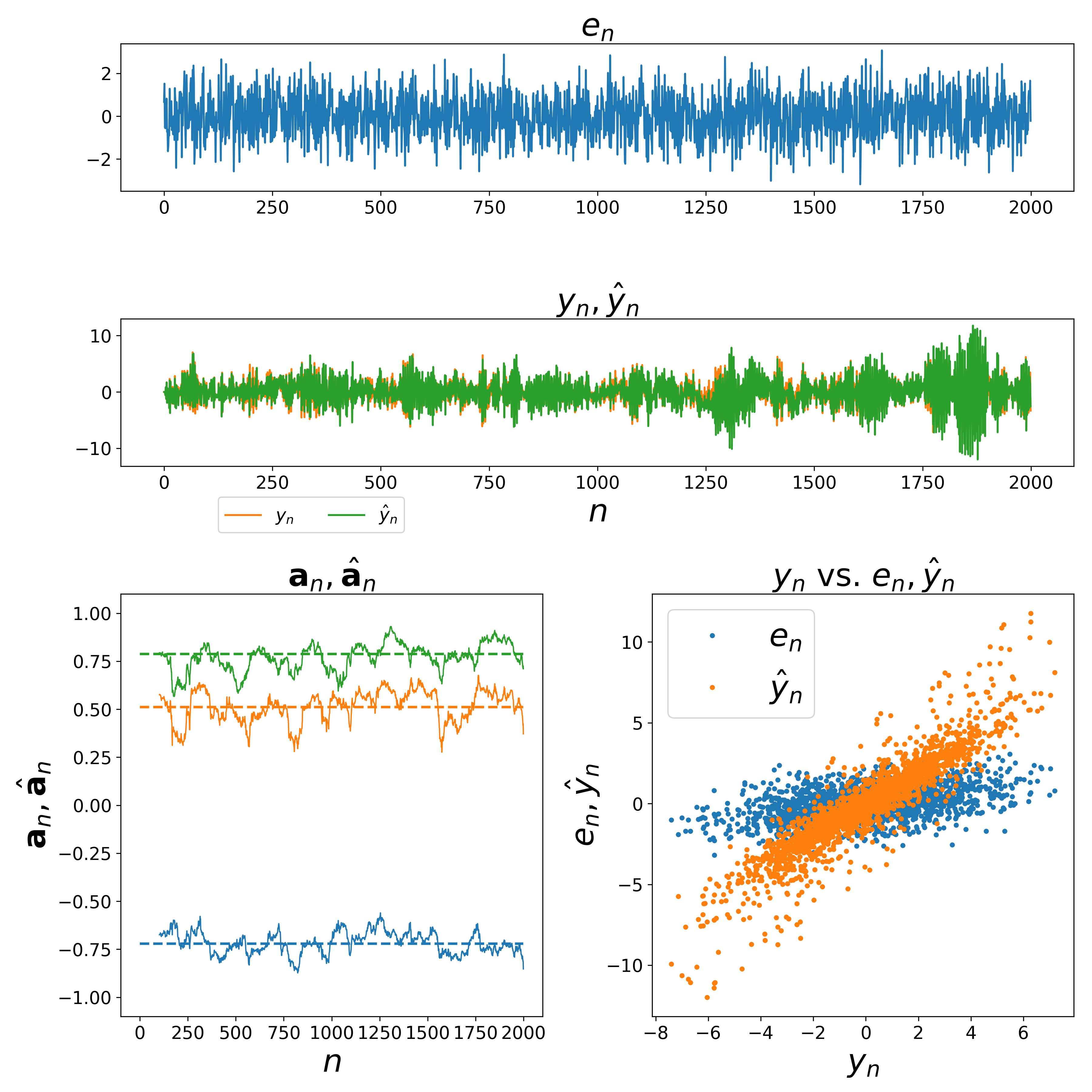
The following figure shows the result from an estimation procedure for a autoregressive process of order 3. The code used for generate this plot can be found here.
Whitening using estimated AR parametes \(\left(\hat{a}\right)\)
Once \(\hat{a}\) is obtained, then the signal \(y_n\) can be whitened by passing it through the following moving average filter.
\[w_n = y_n - \sum_{k=1}^{p} \hat{a}_ky_{n-k}\]\(w_n\) would be the out of this moving average filter, and $w_n$ will be a white noise. The input to this moving average filter the measured time series \(y_n\).