Describing movements with numbers
Movement description beyond words
Movements are changes in the position of an object of interest over time.
Position is a vector quantity describing the spatial location of an object with respect to a chosen reference frame.
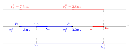
A reference frame is two independent choices: an origin \(O_{A}\) (where \(x=0\) sits) and a basis \(\v{x}_{A}\) (a direction and a length).
With respect to this reference frame \(A\), the positions of particles \(P_1\) and \(P_2\) are given as follows, \[ \v{r}_1^{A} = \m{3.2} \qquad \v{r}_2^{A} = \m{-1.5} \]
where \(\v{r}_{1}^{A}, \v{r}_2^{A} \in \mathbb{R}\). The superscript \(A\) says the position is expressed in reference frame \(A\); the subscripts \(1\) and \(2\) are the particle numbers. A subscript also labels the frame’s own parts, e.g. \(O_A\). The numbers are the coefficients of \(\v{r}\) in the basis of that frame, which here is just \(\v{x}_{A}\).
Who decides the reference frame?
Why did we choose one reference frame over another?
Anyone! We choose what is natural and convenient for the problem at hand.
Both the origin and the basis are fair game.
In this course, we will only choose an orthonormal basis — basis vectors have unit length and are mutually orthogonal.
Reference frame \(B\) is translated and rotated with respect to reference frame \(A\). Every point in the 1D space can be represented in either frame, but the numbers will be different.
Changing between reference frames
How do we change between reference frames?
![]()
Points \(P_1\) and \(P_2\) in the two reference frames.
\[\begin{matrix} \v{r}_1^{A} = \m{3.2} & \v{r}_2^{A} = \m{-1.5} \\ \v{r}_1^{B} = \m{2.8} & \v{r}_2^{B} = \m{7.5} \end{matrix} \]
How are these numbers related?
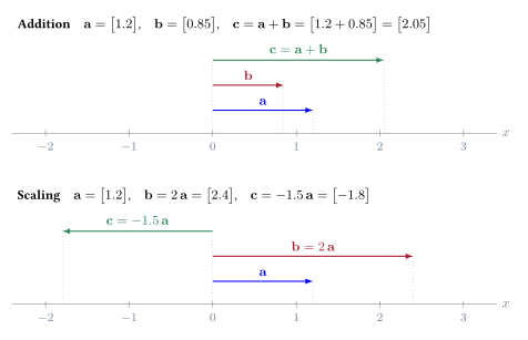
Requires us to do vector addition and scaling.
Changing between reference frames
How do we change between reference frames?
Vector Addition and Scaling in 1D:
Changing between reference frames
How do we change between reference frames?
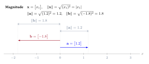
Magnitude of a vector: Also referred to as the 2-norm, Euclidean norm, or length of a vector.
Changing between reference frames
How do we change between reference frames?
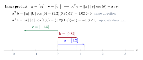
Standard Inner Product between two vectors.
Changing between reference frames
How do we change between reference frames?
![]()
Two pieces of information to change between reference frames:
Rotation of the basis of the target (\(B\)) w.r.t. the base frame (\(A\)). Represented by a rotation matrix \(\v{R}_{B}^{A}\).
Translation of the origin of the target frame (\(B\)) w.r.t. the base frame (\(A\)), represented in the base frame. Represented by a translation vector \(\v{o}_{B}^{A}\).
Changing between reference frames
Rotation Matrix
![]()
Rotation Matrix: \(\v{R}_{B}^{A} \in \mathbb{R}^{1 \times 1}\) — Represents what the basis vectors of the frame \(B\) (subscript) look like in the frame \(A\) (superscript).
\[ \v{R}_{B}^{A} = \m{\v{x}_{A}^\top \v{x}_{B}} \]
In the above example, \(\v{R}_{B}^{A} = \m{-1}\), because \(\Vert \v{x}_A \Vert = 1\), \(\Vert \v{x}_B \Vert = 1\) and \(\theta = 180^\circ\).
Changing between reference frames
Translation Vector
![]()
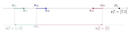
Translation Vector: \(\v{o}_{B}^{A} \in \mathbb{R}^{1 \times 1}\) — Represents the position of the origin of the frame \(B\) (subscript) in the frame \(A\) (superscript). In the above example, \(\v{o}_{B}^{A} = \m{6}\).
The full description of the reference frame \(B\) w.r.t. the reference frame \(A\) is given by the pair \(\left( \v{R}_{B}^{A}, \v{o}_{B}^{A} \right)\).
This pair can be used to transform any vector expressed in frame \(B\) to frame \(A\).
Changing between reference frames
Going back and forth between frames
![]()
Given the pair \(\left( \v{R}_{B}^{A}, \v{o}_{B}^{A} \right)\), we can transform any vector expressed in frame \(B\) to frame \(A\) using the following equation:
\[ \v{r}_{i}^{A} = \v{R}_{B}^{A} \, \v{r}_{i}^{B} + \v{o}_{B}^{A} \]
Product of a matrix with a vector results in a vector.
In 1D, this product is very simple. We simply multiply the individual elements of the matrix and the vector.
Changing between reference frames
Going back and forth between frames
![]()
Given the pair \(\left( \v{R}_{B}^{A}, \v{o}_{B}^{A} \right)\), how do we go the other way around? \(\v{r}_{i}^{A} \mapsto \v{r}_{i}^{B}\).
\[ \v{r}_{i}^{B} = {\v{R}_{B}^{A}}^{-1} \left( \v{r}_{i}^{A} - \v{o}_{B}^{A} \right) = \v{R}_{A}^{B} \v{r}_{i}^{A} + \v{o}_{A}^{B} \]
where, \({\v{R}_{B}^{A}}^{-1} = \v{R}_{A}^{B}\), and \(\v{o}_{A}^{B} = -{\v{R}_{B}^{A}}^{-1}\v{o}_{B}^{A}\).
We obtain \({\v{R}_{B}^{A}}^{-1}\) by inverting the single number in the matrix. So, for the above example, we have, \[ {\v{R}_{B}^{A}}^{-1} = \v{R}_{A}^{B} = \m{\frac{1}{-1}} = \m{-1} \qquad \v{o}_{A}^{B} = -{\v{R}_{B}^{A}}^{-1} \v{o}_{B}^{A} = -\m{-1}\m{6} = \m{6} \]
Changing between reference frames
Going back and forth between frames \(A\) and \(B\)
Given: \(\v{R}_{A}^{B} = \m{-1}\) and \(\v{o}_{A}^{B} = \m{6}\).
Going from \(A\) to \(B\).
\[ P_1: \m{3.2} = \m{-1} \m{2.8} + \m{6} = \m{-2.8} + \m{6} = \m{3.2} \] \[ P_2: \m{-1.5} = \m{-1} \m{7.5} + \m{6} = \m{-7.5} + \m{6} = \m{-1.5} \]
Going from \(B\) to \(A\).
\[ P_1: \m{2.8} = \m{-1} \m{3.2} + \m{6} = \m{-3.2} + \m{6} = \m{2.8} \] \[ P_2: \m{7.5} = \m{-1} \m{-1.5} + \m{6} = \m{1.5} + \m{6} = \m{7.5} \]
Changing between reference frames
Now a third reference frame!
Let’s try a problem by bringing in a third reference frame \(C\).
- Find the pair \(\left( \v{R}_{C}^{A}, \v{o}_{C}^{A} \right)\). \(\longrightarrow \m{1.0}, \m{-2}\)
- Find the pair \(\left( \v{R}_{A}^{C}, \v{o}_{A}^{C} \right)\). \(\longrightarrow \m{1.0}, \m{2}\)
- Find \(\v{r}_{3}^{B}\). \(\longrightarrow \m{-1.5}\)
- Find \(\v{r}_{3}^{C}\). \(\longrightarrow \m{9.5}\)
- Find the pair \(\left( \v{R}_{C}^{B}, \v{o}_{C}^{B} \right)\). \(\longrightarrow \m{-1.0}, \m{8}\)
- Find the pair \(\left( \v{R}_{B}^{C}, \v{o}_{B}^{C} \right)\). \(\longrightarrow \m{-1.0}, \m{8}\)
Describing movements with numbers in 2D
Movement description in 2D
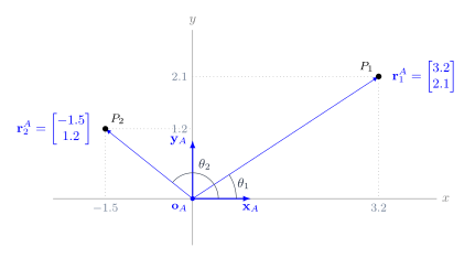
In the 2D real plane, we can represent the position of individual points using two numbers after we choose a reference frame — origin and basis vectors.
Reference frame \(A\): origin \(\v{o}_{A}\) and orthonormal basis \(\{ \v{x}_A, \v{y}_A \}\), where \(\Vert \v{x}_{A} \Vert = \Vert \v{y}_{A} \Vert = 1\) and \(\v{x}_{A}^\top \v{y}_{A} = 0\).
Points in the plane are represented as column vectors \(\v{r}_i^{A} \in \mathbb{R}^2\) w.r.t. the reference frame \(A\). \[ \v{r}_{1}^{A} = \m{ r_{11}^A \\ r_{12}^A} = \m{ \v{x}_A^\top \v{r}_1^{A} \\ \v{y}_A^\top \v{r}_1^{A}} = \m{ \Vert \v{x}_A \Vert \Vert \v{r}_1^{A} \Vert \cos \left( \theta_1 \right) \\ \Vert \v{y}_A \Vert \Vert \v{r}_1^{A} \Vert \sin \left( \theta_1 \right)} = \m{ \Vert \v{r}_1^{A} \Vert \cos \left( \theta_1 \right) \\ \Vert \v{r}_1^{A} \Vert \sin \left( \theta_1 \right)} \]
Describing movements with numbers in 2D
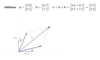
Vector addition in 2D
Vector addition in \(\mathbb{R}^2\)
Describing movements with numbers in 2D
Vector scaling in 2D
Vector scaling in \(\mathbb{R}^2\)
Describing movements with numbers in 2D
Movement description in 2D
The representation of \(P_1\) and \(P_2\) in reference frame \(A\) is \(\v{r}_{1}^{A} = \m{3.2 \\ 2.1}\) and \(\v{r}_{2}^{A} = \m{-1.5 \\ 1.2}\), respectively.
The following is what these numbers mean:
\[ \v{r}_{1}^{A} = 3.2 \v{x}_A + 2.1 \v{y}_A \qquad \qquad \v{r}_{2}^{A} = -1.5 \v{x}_A + 1.2 \v{y}_A\]
Different reference frames in 2D
Reference frame sharing the origin
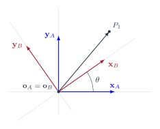
Consider a second reference frame \(B\) shown in the figure. Both these reference frames share the same origin, but are rotated with respect to each other.
Note: \(\Vert \v{x}_{B} \Vert = \Vert \v{y}_{B} \Vert = 1\) and \(\v{x}_{B}^\top\v{y}_{B} = 0\).
The rotation of frame \(B\) with respect to frame \(A\) is given by a \(2 \times 2\) real matrix \(\v{R}_{B}^{A} \in \mathbb{R}^{2 \times 2}\).
\[ \v{R}_{B}^{A} = \m{\v{x}_{B}^{A} & \v{y}_{B}^{A}} = \m{\v{x}_{A}^\top \v{x}_{B} & \v{x}_{A}^\top \v{y}_{B} \\ \v{y}_{A}^\top \v{x}_{B} & \v{y}_{A}^\top \v{y}_{B}}\]
\[ \v{R}_{B}^{A} = \m{ \cos\left( \theta \right) & -\sin\left( \theta \right) \\ \sin\left( \theta \right) & \cos\left( \theta \right) }\]
Representation of \(P_1\) in reference frames \(A\) and \(B\) are \(\v{r}_{1}^{A}\) and \(\v{r}_{1}^{B}\), respectively. \[ \v{r}_{1}^{A} = \m{r_{11}^{A} \\ r_{12}^{A}} \qquad \v{r}_{1}^{B} = \m{r_{11}^{B} \\ r_{12}^{B}} \qquad \v{r}_{1}^{A} = \v{R}_{B}^{A} \, \v{r}_1^{B} \]
The linear algebra we need
Vectors, matrices and a few of their operations
Vectors \(\mathbb{R}^n\) are an ordered collection of real numbers \(\mathbb{R}\). We will also write them as a column and call them column vectors.
\[ \v{x} = \m{x_1 \\ x_2 \\ \vdots \\ x_n} \]
The transpose operation changes a column vector to a row vector and vice versa.
\[ \v{x}^\top = \m{x_1 & x_2 & \cdots & x_n} \qquad \qquad \left(\v{x}^\top\right)^\top = \v{x} \]
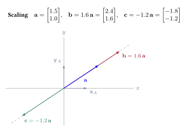
Addition and scaling rules and their geometric interpretation are the same as that in \(\mathbb{R}^2\).
2-Norm: Consider a vector \(\v{x} \in \mathbb{R}^n\). \(\Vert \v{x} \Vert = \sqrt{\sum_{i=1}^n x_i^2 }\)
Standard inner product: Consider two vectors, \(\v{x}, \v{y} \in \mathbb{R}^n\).
\[ \v{x}^\top\v{y} = \m{x_1 & x_2 & \cdots & x_n}\m{y_1 \\ y_2 \\ \vdots \\ y_n} = \sum_{i=1}^n x_iy_i = \Vert \v{x} \Vert \Vert \v{y} \Vert \cos \left(\theta\right)\]
where, \(\theta\) is the angle between \(\v{x}\) and \(\v{y}\).
The linear algebra we need
Vectors, matrices and a few of their operations
Matrices \(\mathbb{R}^{p \times q}\) are a rectangular arrangement of numbers \(\mathbb{R}\).
\[ \v{A} = \m{a_{11} & a_{12} & \cdots & a_{1q} \\
a_{21} & a_{22} & \cdots & a_{2q} \\
\vdots & \vdots & \ddots & \vdots \\
a_{p1} & a_{p2} & \cdots & a_{pq}} \in \mathbb{R}^{p \times q}\]
where, \(a_{ij}\) is the component of the matrix in the \(i^{th}\) row and \(j^{th}\) column. When \(p = q\), \(\v{A}\) is a square matrix, else it’s a rectangular matrix.
With this definition, we can think of column vectors as a matrix with a single column, and a row vector as a matrix with a single row.
We can also think of the matrix \(\v{A}\) as a row of column vectors from \(\mathbb{R}^p\).
\[ \v{A} = \m{\v{a}_{1} & \v{a}_{2} & \cdots & \v{a}_{q}} \in \mathbb{R}^{p \times q}\]
where, \(\v{a}_{i} \in \mathbb{R}^p\) is the \(i^{th}\) column of \(\v{A}\).
Transpose of a matrix switches the rows and columns. \(\v{A}^\top \in \mathbb{R}^{q \times p}\).
\[ \v{A}^\top = \m{a_{11} & a_{21} & \cdots & a_{p1} \\
a_{12} & a_{22} & \cdots & a_{p2} \\
\vdots & \vdots & \ddots & \vdots \\
a_{1q} & a_{2q} & \cdots & a_{pq}} \in \mathbb{R}^{q \times p}\]
The linear algebra we need
Vectors, matrices and a few of their operations
Matrix-vector product Let \(\v{A} \in \mathbb{R}^{p \times q}\) and \(\v{x} \in \mathbb{R}^{q \times 1}\). We can define this product as the following,
\[ \mathbb{R}^{p} \ni \v{y} = \v{A}\v{x}
= \m{a_{11} & a_{12} & \cdots & a_{1q} \\
a_{21} & a_{22} & \cdots & a_{2q} \\
\vdots & \vdots & \ddots & \vdots \\
a_{p1} & a_{p2} & \cdots & a_{pq}} \m{x_1 \\ x_2 \\ \vdots \\ x_q} = \m{\sum_{i=1}^qa_{1i} x_i \\ \sum_{i=1}^qa_{2i} x_i \\ \vdots \\ \sum_{i=1}^qa_{pi} x_i}\]
We can also view \(\v{A}\v{x}\) as the following,
\[ \v{y} = \v{A}\v{x}
= \m{\v{a}_{1} & \v{a}_{2} & \cdots & \v{a}_{q}} \m{x_1 \\ x_2 \\ \vdots \\ x_q} = \sum_{i=1}^q x_i \v{a}_{i}\]
Matrix-Matrix product Let \(\v{A} \in \mathbb{R}^{p \times q}\) and \(\v{B} \in \mathbb{R}^{q \times r}\). Then we can define the product of these two matrices as the following,
\[ \mathbb{R}^{p \times r} \ni \v{C}
= \m{c_{11} & c_{12} & \cdots & c_{1r} \\
c_{21} & c_{22} & \cdots & c_{2r} \\
\vdots & \vdots & \ddots & \vdots \\
c_{p1} & c_{p2} & \cdots & c_{pr}}
= \v{A}\v{B}
= \m{a_{11} & a_{12} & \cdots & a_{1q} \\
a_{21} & a_{22} & \cdots & a_{2q} \\
\vdots & \vdots & \ddots & \vdots \\
a_{p1} & a_{p2} & \cdots & a_{pq}}
\m{b_{11} & b_{12} & \cdots & b_{1r} \\
b_{21} & b_{22} & \cdots & b_{2r} \\
\vdots & \vdots & \ddots & \vdots \\
b_{q1} & b_{q2} & \cdots & b_{qr}} \qquad c_{ij} = \sum_{k} a_{ik}b_{kj}\]
Matrix multiplication \(\v{A}\v{B}\) is allowed if and only if the number of columns of \(\v{A}\) equals the number of rows of \(\v{B}\).
Different reference frames in 2D
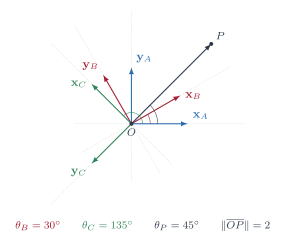
Let’s do an example
Find the following.
- \(\v{r}_{P}^{A}\). \(\longrightarrow \m{\sqrt{2} \\ \sqrt{2}}\)
- \(\v{R}_{B}^{A}\). \(\longrightarrow \frac{1}{2}\m{\sqrt{3} & -1 \\ 1 & \sqrt{3}}\)
- \(\v{R}_{A}^{B}\). \(\longrightarrow \frac{1}{2}\m{\sqrt{3} & 1 \\ -1 & \sqrt{3}}\)
- \(\v{R}_{C}^{A}\). \(\longrightarrow \frac{1}{\sqrt{2}}\m{-1 & -1 \\ 1 & -1}\)
- \(\v{R}_{A}^{C}\). \(\longrightarrow \frac{1}{\sqrt{2}}\m{-1 & 1 \\ -1 & -1}\)
- \(\v{r}_{P}^{B}\). \(\longrightarrow \frac{1}{2}\m{\sqrt{6}+\sqrt{2} \\ \sqrt{6}-\sqrt{2}}\)
- \(\v{r}_{P}^{C}\). \(\longrightarrow \m{0 \\ -2}\)
- \(\v{R}_{B}^{C}\). \(\longrightarrow \frac{1}{4}\m{\sqrt{2}-\sqrt{6} & \sqrt{6}+\sqrt{2} \\ -\sqrt{6}-\sqrt{2} & \sqrt{2}-\sqrt{6}}\)
- \(\v{R}_{C}^{B}\). \(\longrightarrow \frac{1}{4}\m{\sqrt{2}-\sqrt{6} & -\sqrt{6}-\sqrt{2} \\ \sqrt{6}+\sqrt{2} & \sqrt{2}-\sqrt{6}}\)
Different reference frames in 2D
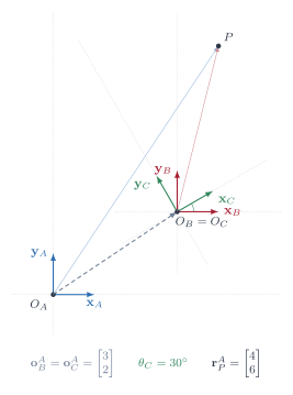
Let’s now shift the origin
What is \(\v{R}_{B}^{A}\)? \(\longrightarrow \m{1 & 0 \\ 0 & 1} = \v{I}\)
What is \(\v{r}_{P}^{B}\)? \(\longrightarrow \m{1 \\ 4}\)
What is \(\v{R}_{C}^{B}\)? \(\longrightarrow \m{\frac{\sqrt{3}}{2} & -\frac{1}{2} \\ \frac{1}{2} & \frac{\sqrt{3}}{2}}\)
How do we change between reference frames \(A\) and \(B\)? We have rotation and the translation. \(\left( \v{R}_{B}^{A}, \v{o}_{B}^{A}\right)\).
\[ \v{r}_{P}^{A} = \v{R}_{B}^{A} \v{r}_{P}^{B} + \v{o}_{B}^{A} \] \[ \v{r}_{P}^{B} = {\v{R}_{B}^{A}}^{-1} \left( \v{r}_{P}^{A} - \v{o}_{B}^{A} \right) \]
\[\implies \v{R}_{A}^{B} = {\v{R}_{B}^{A}}^{-1} = {\v{R}_{B}^{A}}^{\top} \qquad \v{o}_{A}^{B} = -{\v{R}_{B}^{A}}^{\top}\v{o}_{B}^{A}\]
Different reference frames in 2D
Let’s now shift the origin
What is \(\v{r}_{P}^{C}\) if we know \(\v{r}_P^{B}\)?
We need \(\left( \v{R}_{C}^{B}, \v{o}_{C}^{B}\right) \longrightarrow \v{r}_{P}^{C} = \v{R}_{B}^{C} \left(\v{r}_{P}^{B} - \v{o}_{C}^{B} \right)\)
\[\v{r}_{P}^{C} = \m{\frac{\sqrt{3}}{2} + 2 \\ -\frac{1}{2} + 2\sqrt{3}}\]
What is \(\v{r}_{P}^{C}\) if we know \(\v{r}_P^{A}\)?
We need \(\left( \v{R}_{C}^{A}, \v{o}_{C}^{A}\right)\)
\[\v{R}_{C}^{A} = \v{R}_{B}^{A}\v{R}_{C}^{B} \qquad \v{o}_{C}^{A} = \v{o}_{B}^{A} + \v{R}_{B}^{A} \v{o}_{C}^{B}\]
\[\v{r}_{P}^{C} = \v{R}_{A}^{C}\left(\v{r}_{P}^{A} - \v{o}_{C}^{A}\right)\]
What is \(\v{r}_{P}^{C}\), if \(\v{o}_{C}^{B} = \m{1 \\ 1}\)? \(\v{r}_{P}^{C} = \m{\frac{3}{2} \\ \frac{3\sqrt{3}}{2}}\)
Different reference frames in 2D
Homogeneous Coordinates
\[ \v{r}_{P}^{A} = \v{R}_{B}^{A} \v{r}_{P}^{B} + \v{o}_{B}^{A} \qquad \qquad \v{r}_{P}^{B} = {\v{R}_{B}^{A}}^{\top} \left( \v{r}_{P}^{A} - \v{o}_{B}^{A} \right) \]
Note that rotation is represented by a matrix multiplication operation, while translation is represented by vector addition.
Homogeneous coordinates
We can express this entire transformation through a multiplication operation if we choose the homogeneous coordinate representation.
Let \(\tilde{\v{r}}_{P}^{C}\) be the homogeneous coordinates of the point \(P\) in reference frame \(C\): \(\quad \tilde{\v{r}}_{P}^{C} = \m{\v{r}_{P}^{C} \\ 1}\).
Note that an \(n\)-dimensional vector is represented by an \((n+1)\)-dimensional vector in the homogeneous coordinates.
In the homogeneous coordinates, there are infinitely many ways to represent the same point.
\[\m{x \\ y \\ z \\ 1} \;{\Large\equiv}\; \m{\lambda x \\ \lambda y \\ \lambda z \\ \lambda}\]
Different reference frames in 2D
Homogeneous Transformation
Homogeneous transformation
Both translation and rotation have a matrix representation – homogeneous transformation matrix.
The homogeneous transformation matrix representing frame \(C\) w.r.t. \(A\) is given by, \(\v{H}_{C}^{A} = \m{\v{R}_{C}^{A} & \v{o}_{C}^{A} \\ \v{0} & 1}\)
We can obtain the homogeneous representation of \(P\) in \(A\) from \(\v{r}_{P}^{C}\) as follows,
\[ \tilde{\v{r}}_{P}^{A} = \v{H}_{C}^{A} \tilde{\v{r}}_{P}^{C} \quad \implies \quad \tilde{\v{r}}_{P}^{C} = \v{H}_{A}^{C} \tilde{\v{r}}_{P}^{A} = {\v{H}_{C}^{A}}^{-1} \tilde{\v{r}}_{P}^{A}\]
What is \({\v{H}_{C}^{A}}^{-1}\)? \(\longrightarrow \m{{\v{R}_{C}^{A}}^\top & -{\v{R}_{C}^{A}}^\top \v{o}_{C}^{A} \\ \v{0} & 1}\)
Different reference frames in 3D
Ideas from 2D generalize to 3D
Each coordinate is an inner product: drop a perpendicular onto that axis, and the length you cut off is \(\v{x}_{A}^\top \v{r}_{P}^{A}\).
Different reference frames in 3D
Ideas from 2D generalize to 3D
Two reference frames, rotated and translated with respect to each other. The same point \(P\) — two sets of numbers. Switch which frame the world is drawn in: the picture changes, the numbers do not.
Different reference frames in 3D
Ideas from 2D generalize to 3D
The representation of a reference frame \(B\) w.r.t. \(A\) requires the rotation matrix \(\v{R}_{B}^{A}\) and the translation of the origin \(\v{o}_{B}^{A} \in \mathbb{R}^3\).
\[ \v{R}_{B}^{A} = \m{
\v{x}_{A}^\top \v{x}_B & \v{x}_{A}^\top \v{y}_B & \v{x}_{A}^\top \v{z}_B \\
\v{y}_{A}^\top \v{x}_B & \v{y}_{A}^\top \v{y}_B & \v{y}_{A}^\top \v{z}_B \\
\v{z}_{A}^\top \v{x}_B & \v{z}_{A}^\top \v{y}_B & \v{z}_{A}^\top \v{z}_B} \in \mathbb{R}^{3 \times 3}\]
The transformation between \(A\) and \(B\) is given by the following,
\[ \v{r}_{P}^{A} = \v{R}_{B}^{A} \v{r}_{P}^{B} + \v{o}_{B}^{A} \qquad \qquad \v{r}_{P}^{B} = {\v{R}_{B}^{A}}^{\top} \left( \v{r}_{P}^{A} - \v{o}_{B}^{A} \right) \]
In the homogeneous representation, we have \(\tilde{\v{r}}_{P}^{B} = \m{\v{r}_{P}^{B} \\ 1}\). And the homogeneous transformation matrix \(\v{H}_{B}^{A} \in \mathbb{R}^{4 \times 4}\).
\[\tilde{\v{r}}_{P}^{A} = \v{H}_{B}^{A} \tilde{\v{r}}_{P}^{B} \quad \implies \quad \tilde{\v{r}}_{P}^{B} = \v{H}_{A}^{B} \tilde{\v{r}}_{P}^{A} = {\v{H}_{B}^{A}}^{-1} \tilde{\v{r}}_{P}^{A}\]
Representing kinematics of rigid bodies
How many numbers do we need?
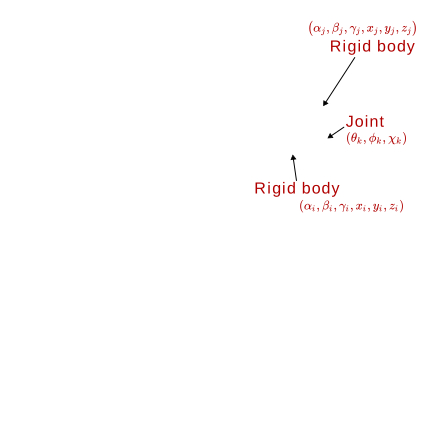
A rigid body is a collection of points whose relative spatial location with respect to each other does not change no matter the forces acting on these points.
Useful approximation for many applications, simplifying representing/analysing kinematics of real objects.
We need a total of 6 numbers to represent its position and orientation w.r.t. a reference frame.
\[ \text{Rigid body in 3D space} \longrightarrow \left( \alpha, \beta, \gamma, x, y, z\right)\]
\(\left(\alpha, \beta, \gamma\right)\) represent the orientation of the body in space, and \(\left(x, y, z\right)\) represents, typically, the position of some point in the rigid body. Once we know these 6 numbers, we know (i.e. can compute) the location of every point in the rigid body.
One of many ways to describe rigid body kinematics in 3D space; all representations need 6 numbers.
These numbers are also referred to as degrees-of-freedom (DOFs).
Representing kinematics of rigid bodies
How many numbers do we need?
Representing kinematics of connected rigid bodies
How many numbers for connected rigid bodies?
If we have two independent rigid bodies in space, how many numbers do we need to describe their kinematics in 3D space? 12
When we say two rigid bodies are connected together, we mean that the two bodies have constraints on how they can move with respect to each other.
Reduces the numbers we need to describe the kinematics of the connected rigid bodies to be lower than 12.
Each constraint on the movements of the two connected bodies reduces the number of DOFs by 1.
\[\text{DOFs of two connected rigid bodies} = 12 - \text{No. of kinematic constraints}\]
We will refer to this connection as a joint, and we can talk about the DOFs of a joint.
\[\text{DOFs of a joint} = 6 - \text{No. of kinematic constraints}\]
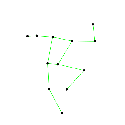
The body as connected rigid bodies
Full body kinematics: Track one body segment and the joint angles of the connected segments.
Individual joint kinematics: Track only the segments connected at the joints.
How do we measure kinematics?
General approach: track all 6DOFs of each limb segment \(\longrightarrow\) derive the individual joint variables.
- Pros: Full characterisation; Suitable for complex movement behaviors (e.g. gait analysis, upper-limb reaching, object manipulation, etc.).
- Cons: Too much information for simple movements (e.g. knee flexion/extension, elbow range of motion); Complex, expensive tools required.
Joint level approach: track specific joint variables of interest.
- Pros: Simple, compact tools. Focused, relevant information for simple movements.
- Cons: Unsuitable for complex movements.
We will explore sensing tools for both approaches.
- Camera-based motion tracking with markers (standard & fiducial).
- Inertial measurement units
- Optical and magnetic encoders
Camera-based movement tracking
![]()
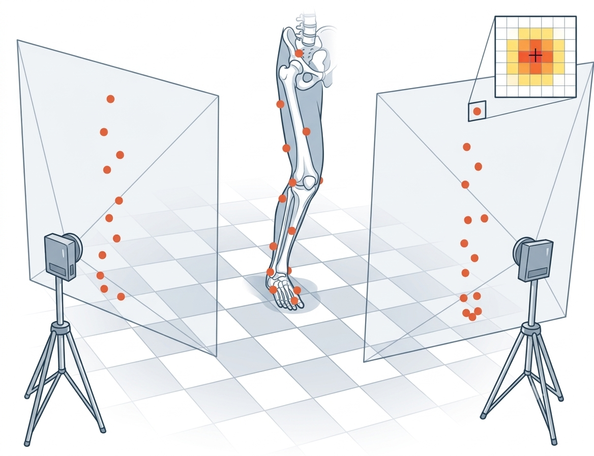
- Each marker is treated as a dot or point in space.
- \((x_i, y_i, z_i)\) position of the \(i^{th}\) marker estimated from the cameras in a lab-fixed reference frame.
\[ \left(x_i, y_i, z_i \right)_{i=1}^{M} \longrightarrow \left(x_j, y_j, z_j, \alpha_j, \beta_j, \gamma_j \right)_{j=1}^{L} \longrightarrow \left(\theta_k, \phi_k, \chi_k \right)_{k=1}^{J}\]
Camera-based movement tracking
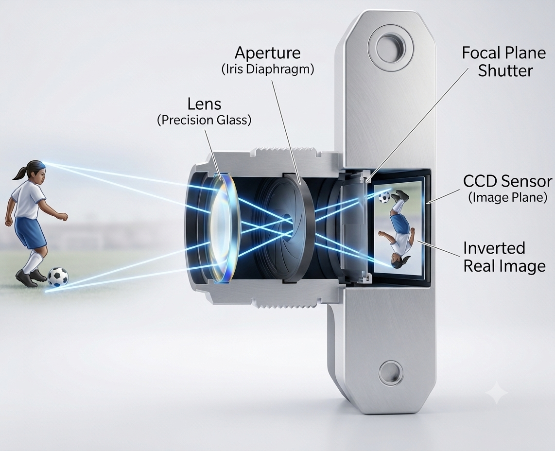
A camera captures the spatial distribution of light arriving from the environment — it records the direction from which light arrives, not the distance it has travelled.
Camera optics produce an image of the world, captured by an image sensor (CCD or CMOS) in digital cameras, or by film in traditional cameras.
An image \(I\left(x, y\right)\) is a 2D distribution of brightness of light. For a camera, the 2D surface is a rectangular region \(\Omega\). \[ I: \Omega \subset \mathbb{R}^2 \mapsto \mathbb{R}_{+}; \quad \Omega \ni \left(x, y\right) \mapsto I\left(x, y\right) \in \mathbb{R}_{+} \]
Image intensity \(I\left(x, y\right)\) at any location \(\left(x, y\right)\) is determined by the amount of light entering the camera through its optical system that directs the light to the image sensor.
Geometry of the optics determines the mapping of the spatial location of a source of light in the world \(\left(x^W, y^W, z^W\right)\) to a spatial location of the image \(\left(x^I, y^I\right)\).
We will primarily focus on the geometry of the optics for the purpose of kinematics tracking using camera image.
Camera-based movement tracking
Physics of a Pinhole Camera
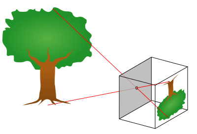
A useful and simplified model of the geometry of a camera’s optics is provided by a pinhole camera.
A box with an infinitesimally small hole that lets only a single ray from each point enter the box.
Produces an inverted image of the world on the back wall.
Camera-based movement tracking
Physics of a Pinhole Camera
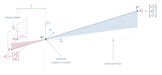
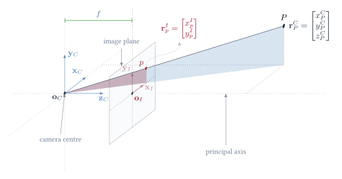
\(P\) in space has coordinates \(\v{r}_P^C = \m{x_P^C & y_P^C & z_P^C}^\top \in \mathbb{R}^3\) w.r.t. the camera reference frame.
\(p\) is the corresponding point in the image with coordinates \(\v{r}_p^I = \m{x_p^I & y_p^I}^\top \in \mathbb{R}^2\) w.r.t. the image reference frame.
\(\mathbf{o}_I\) is principal point of the image, i.e. the point where the optical axis intersects the image plane.
Camera-based movement tracking
Physics of a Pinhole Camera
Assume the image plane to be in front of the camera center, then we have,
\[x_p^I = \frac{f}{z_P^C} x_P^C \qquad y_p^I = \frac{f}{z_P^C} y_P^C \implies z_P^C \m{x_p^I \\ y_p^I \\ 1} = \m{f & 0 & 0 & 0\\ 0 & f & 0 & 0\\ 0 & 0 & 1 & 0}\m{x_P^C \\ y_P^C \\ z_P^C \\ 1}\]
Camera-based movement tracking
Physics of a Pinhole Camera
\[x_p^I = \frac{f}{z_P^C} x_P^C \qquad y_p^I = \frac{f}{z_P^C} y_P^C\] \[\v{r}_p^I = \m{x_p^I \\ y_p^I \\ 1} \equiv \m{f x_P^C \\ f y_P^C \\ z_P^C} = \m{f & 0 & 0 & 0\\ 0 & f & 0 & 0\\ 0 & 0 & 1 & 0}\m{x_P^C \\ y_P^C \\ z_P^C \\ 1}\]
We can now split this into two matrices,
\[\m{f & 0 & 0 & 0\\ 0 & f & 0 & 0\\ 0 & 0 & 1 & 0} = \m{f & 0 & 0\\ 0 & f & 0\\ 0 & 0 & 1} \m{1 & 0 & 0 & 0\\ 0 & 1 & 0 & 0\\ 0 & 0 & 1 & 0} = \m{f & 0 & 0\\ 0 & f & 0\\ 0 & 0 & 1} \m{\v{I}_3 & \v{0}}\]
\[\v{r}_p^I = \m{f & 0 & 0\\ 0 & f & 0\\ 0 & 0 & 1} \m{\v{I}_3 & \v{0}} \v{r}_P^C\]
Note: we will drop the \(\,\, \tilde{} \,\,\) symbol for vectors since we will mostly deal with homogeneous coordinates in this section.
Camera-based movement tracking
Physics of a Pinhole Camera
If the point \(P\) is represented with respect to a world coordinate frame \(W\) represented by \(\left( \v{R}_{W}^{C}, \v{o}_{W}^{C}\right)\), then we have,
\[\v{r}_P^C = \m{\v{R}_{W}^{C} & \v{o}_{W}^{C} \\ \v{0} & 1} \v{r}_P^W\]
\[\implies \v{r}_p^I = \m{f & 0 & 0\\ 0 & f & 0\\ 0 & 0 & 1} \m{\v{I}_3 & \v{0}} \m{\v{R}_{W}^{C} & \v{o}_{W}^{C} \\ \v{0} & 1} \v{r}_P^W = \m{f & 0 & 0\\ 0 & f & 0\\ 0 & 0 & 1} \m{\v{R}_{W}^{C} & \v{o}_{W}^{C}} \v{r}_P^W\]
The 6 parameters associated with the transformation between the world \(W\) and the camera \(C\) reference frames are called the extrinsic parameters of the camera.
Camera-based movement tracking
Physics of a Pinhole Camera
Camera-based movement tracking
Physics of a Pinhole Camera
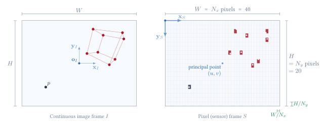
With digital cameras, positions on an image are reported in pixels. Each pixel corresponds to a sensing area on the image plane.
We need to convert from \(\v{r}_p^I\) (e.g. units of mm) to sensor coordinates \(\v{r}_p^S\) in pixels.
The origin and the coordinate axes for the sensor frame \(S\) can be different.
How do we convert from \(\v{r}_p^I\) to \(\v{r}_p^S\)?
Camera-based movement tracking
Physics of a Pinhole Camera
How do we convert from \(\v{r}_p^I\) to \(\v{r}_p^S\)?
\[\v{r}_p^S = \m{s_x & s_{\theta} & 0 \\ 0 & s_y & 0 \\ 0 & 0 & 1} \m{1 & 0 & u \\ 0 & -1 & v \\ 0 & 0 & 1} \v{r}_p^I\]
\[\begin{align} x_p^S &= s_x\left(x_p^I + u\right) + s_\theta \left(-y_p^I + v\right) \\
y_p^S &= s_y\left(-y_p^I + v\right)
\end{align}\]
\[\v{r}_p^S = \m{s_x & s_{\theta} & 0 \\ 0 & s_y & 0 \\ 0 & 0 & 1} \m{1 & 0 & u \\ 0 & -1 & v \\ 0 & 0 & 1} \m{f & 0 & 0\\ 0 & f & 0\\ 0 & 0 & 1} \m{\v{R}_{W}^{C} & \v{o}_{W}^{C}} \v{r}_P^W = \v{K}_f \m{\v{R}_{W}^{C} & \v{o}_{W}^{C}} \v{r}_P^W\]
Looks like there are additional 6 parameters associated with the camera itself – \(\left(f, s_x, s_y, s_\theta, u, v\right)\). But there are only 5!
\[\v{K}_f = \m{s_x f & -s_{\theta} f & s_x u + s_\theta v \\ 0 & -s_y f & s_y v \\ 0 & 0 & 1}\]
Camera-based movement tracking
Physics of a Pinhole Camera
Camera-based movement tracking
Physics of a Pinhole Camera
The full camera image formation model for the pinhole camera is given by,
\[\v{r}_p^S = \v{K}_f \m{\v{R}_{W}^{C} & \v{o}_{W}^{C}} \v{r}_P^W, \qquad \v{K}_f = \m{f_x & s & o_{xs} \\ 0 & f_y & o_{ys} \\ 0 & 0 & 1 }\]
where,
- \(f_x\) is the focal length in horizontal pixels.
- \(f_y\) is the focal length in vertical pixels.
- \(s\) is the skew when the sensor’s rows and columns are not perpendicular.
- \(o_{xs}\) is the principal point’s horizontal location in pixels.
- \(o_{ys}\) is the principal point’s vertical location in pixels.
These are the 5 intrinsic parameters of the camera.
We need to know all 11 parameters to know the full mapping from 3D coordinates to image coordinates in pixels.
These are obtained through a camera calibration procedure.
Camera-based movement tracking
Camera distortion
Real cameras are not pinhole cameras. They employ lenses to collect more light for producing brighter images.
Lenses introduce different types of distortions on images. The most common distortions considered are: (a) radial distortion or barrel distortion, and (b) tangential distortion
The distortion acts before the pixel conversion, on the normalised coordinates \(\v{r}_p^N\) — centred on the optical axis and divided by \(z_P^C\), so they carry no units:
\[\m{{x_p^N} \\ {y_p^N}} = \frac{1}{z_P^C}\m{x_P^C \\ y_P^C}, \qquad r^2 = {x_p^N}^2 + {y_p^N}^2\]
\[\v{r}_p^D = \v{f}_d\left( \v{r}_p^N \right) =
\underbrace{\left(1 + k_1 r^2 + k_2 r^4 + k_3 r^6\right)\m{{x_p^N} \\ {y_p^N}}}_{\textrm{radial}}
+ \underbrace{\m{2 p_1 {x_p^N} {y_p^N} + p_2 \left(r^2 + 2{x_p^N}^2\right) \\ p_1\left(r^2 + 2{y_p^N}^2\right) + 2 p_2 {x_p^N} {y_p^N}}}_{\textrm{tangential}}\]
\[\v{r}_p^S = \v{K}_f \, \v{r}_p^D \qquad \textrm{— only now do we get pixels}\]
Camera-based movement tracking
Camera distortion
Camera-based movement tracking
Camera calibration
Camera image formation model \[\v{r}_p^S = \underbrace{\v{K}_f}_{\textrm{5 intrinsic}} \underbrace{\m{\v{R}_{W}^{C} & \v{o}_{W}^{C}}}_{\textrm{6 extrinsic}} \v{r}_P^W = \boldsymbol{\Pi} \v{r}_P^W\]
Intrinsic — properties of the camera itself. Measured once, valid until someone changes the lens or the zoom.
Extrinsic — where the camera is. Changes the moment anyone moves it.
Calibration is how we get numbers in the above model.
The idea behind every method is the same:
- put objects of known geometry in front of the camera.
- find them in the image.
- ask which numbers would have produced the picture we actually got.
Camera-based movement tracking
Camera calibration — Direct Linear Transform
The oldest and simplest approach — solve for all 11 numbers of \(\boldsymbol{\Pi}\) in one step.
You provide
- A 3D object whose points you have measured — a calibration frame or jig.
- At least 6 points, and their positions in the image.
- The points must not all lie on a plane.
The software returns
- \(\boldsymbol{\Pi}\), the whole \(3 \times 4\) matrix, up to scale.
- From which the intrinsics and extrinsics can be separated.
Each point gives two equations — one for its row, one for its column in the image. Six points give twelve, which is enough for eleven unknowns.
Issues with the method
- Requires a measured calibration object with known, non-coplanar points that fill the capture volume — estimates extrapolate poorly outside it.
- Ignores lens distortion — unmodelled distortion biases all 11 parameters.
- Fits 11 free parameters without enforcing the structure of \(\boldsymbol{\Pi} = \v{K}\m{\v{R} \mid \v{o}}\) (orthogonal \(\v{R}\)), so the spare degrees of freedom absorb measurement noise.
- Minimises algebraic rather than reprojection error; needs data normalisation to be well-conditioned.
Camera-based movement tracking
Camera calibration — Zhang’s method
The method every calibration tool uses. It needs only a flat printed target — no machined 3D rig.
You provide
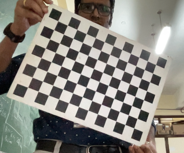
- A checkered board of known square size.
- Many photographs of it — 15 to 20 — held at different tilts, distances, and positions in the frame.
The software returns
- The 5 intrinsic parameters.
- The distortion parameters \(k_1, k_2, k_3, p_1, p_2\).
- Where the board was in each photograph.
How it decides:
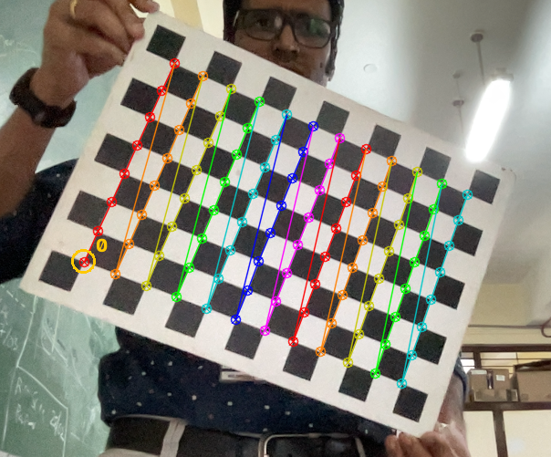
- positions of the corners on the checkered board are known.
- detects the corners for the given size; this provides the correspondence between the 3D points and the image points.
- searches for the set of numbers that best predicts where every corner actually appeared
- leftover mismatch, in pixels, is the reprojection error.
Camera-based movement tracking
Camera calibration — what to check
Calibration always returns numbers. It never refuses. So the question is never “did it run?” but “should I believe it?”
- Were the boards tilted? Images with the board parallel to the camera carry the same information over and over — the fit becomes ill-conditioned.
- Did the board reach the corners of the frame? Distortion is largest at the edges. Calibrate only from the middle of the image and the distortion parameters are guesswork.
- Was the board actually flat? Paper on a clipboard curls. The method assumes a plane, and a bent target quietly biases every number.
- Is the square size right? Get it wrong and the intrinsics are unaffected, but every distance you go on to measure is scaled by the same factor.
- How large is the reprojection error? Typically well under half a pixel. But a low error on a bad set of images means the model fits those images — not that the camera is characterised.
A small residual is necessary, not sufficient. This is the same lesson as static calibration in Module 1 — the fit quality tells you about the fit, not about the instrument.
Camera-based movement tracking
Single camera inverse problem
Can we estimate the position of points in 3D space from a single camera?
Let’s assume that we have calibrated the camera. \(\v{K}\) is estimated and \(\v{R} = \v{I}\) and \(\v{o} = \v{0}\) assuming camera coordinate is the world coordinate.
Forward problem: 3D point \(\v{r}_P^W\) in world to 2D point in the image \(\v{r}_p^S\). \[\lambda \v{r}_p^S = \v{K}_f \m{\v{I}_3 & \v{0}} \v{r}_P^W\]
\(\lambda > 0\) is an unknown here because we are operating with homogeneous coordinates, and \(\v{r}_p^S = \m{x_p^S \\ y_p^S \\ 1}\).
Inverse problem: Knowing \(\v{r}_p^S\), we would like to find the 3D points that would have produced it.
We can now invert the relationship to find the following,
\[ \v{r}_P^W = \lambda \v{K}_f^{-1} \v{r}_p^S \]
This is the equation of a ray from the camera’s origin, pointing in the direction \(\v{K}_f^{-1} \v{r}_p^S\) !
Camera-based movement tracking
Single camera inverse problem
Camera-based movement tracking
Two cameras can solve the inverse problem
What if we have the image locations of the same point from two or more cameras?
It turns out that you can now solve for the 3D location, as long as the two camera centres do not coincide.
This way there are two rays starting at two different locations, and their intersection is the 3D point of interest!
We, of course, assume the ideal scenario here.
In the real scenario, we can only estimate the location of the 3D point using a least squares approach.
Camera-based movement tracking
Two cameras — the forward problem
Forward problem: 3D point \(\v{r}_P^W\) in world to the 2D points in the two images \(\v{r}_p^{S_A}\) and \(\v{r}_p^{S_B}\) in cameras \(A\) and \(B\), respectively.
Assumption: (a) Camera \(A\) as the world reference frame, and (b) Camera \(A\)’s frame known w.r.t. camera \(B\), \(\left(\v{R}_{A}^{B}, \v{o}_{A}^{B}\right)\).
Then the forward problem is as follows, \[\lambda_a \v{r}_p^{S_A} = \v{K}_{f}^{A} \m{\v{I}_3 & \v{0}} \v{r}_P^W \qquad \lambda_b \v{r}_p^{S_B} = \v{K}_{f}^{B} \m{\v{R}_{A}^{B} & \v{o}_{A}^{B}} \v{r}_P^W \]
\(\lambda_a, \lambda_b > 0\) are unknowns, and \(\v{r}_p^{S_A} = \m{x_p^{S_A} & y_p^{S_A} & 1}^\top, \v{r}_p^{S_B} = \m{x_p^{S_B} & y_p^{S_B} & 1}^\top\)
What are the \(\lambda\) s? These are the depths of the 3D point for each camera!
\(x_p^{S_A}, y_p^{S_A}\) and \(x_p^{S_B}, y_p^{S_B}\): sensor coordinates in the images from cameras \(A\) and \(B\), respectively.
There are 6 equations (3 for each camera) and 5 unknowns \(\left(x_P^W, y_P^W, z_P^W, \lambda_a, \lambda_b\right)\).
Camera-based movement tracking
Two cameras — finding the point
Camera-based movement tracking
Practical issues
Our discussion, thus far, has entirely focused on the ideal scenario.
In practice there are several issues that require careful consideration.
- Spatial sampling of the image plane: a point’s image is located only to within a fraction of a pixel, and that error grows with distance from the camera.
- Image sensor noise: noise moves the detected centre from frame to frame, so a still marker appears to jitter.
- Image distortion: removed by calibration — what is left is only as good as the calibration.
- Identification of corresponding points: which blob is which marker, in every camera and every frame? Swapped labels corrupt the data without any warning.
- Temporal synchronization between cameras: unsynchronized cameras see a moving point at different times, so the rays do not meet. The error grows with speed.
Camera-based movement tracking
Human movement tracking setup
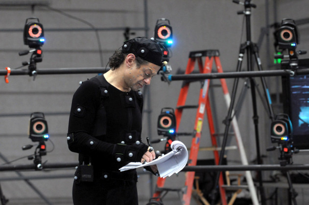
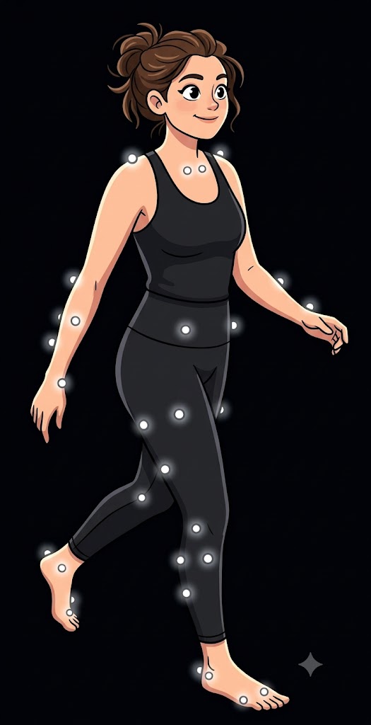
Tracking full body kinematics typically involves markers placed on the individual body segments, which are then tracked using a multi-camera setup.
Each rigid body has 3-4 markers to track its pose in 3D.