Everyone that has taken linear algebra is quite comfortable with the idea of the standard inner product between two vectors \(\mathbf{x}, \mathbf{y} \in \mathbb{R}^n\).
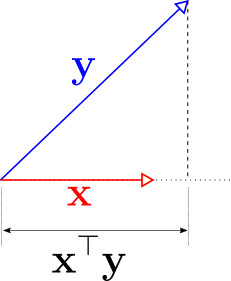
\[\mathbf{x}^\top\mathbf{y} = \begin{bmatrix} x_1 & x_2 & \cdots & x_n\end{bmatrix}\begin{bmatrix} y_1 \\ y_2 \\ \vdots \\ y_n\end{bmatrix} = \sum_{i=0}^nx_i\cdot y_i \in \mathbb{R}\]This is the dot product we use in high school physics and mathematics. This has a nice geometric interpretation as shown in the following figure, where we assume that vector \(\mathbf{x}\) is of unit length, i.e. \(\mathbf{x}^\top\mathbf{x} = 1\).
We could this of the number \(\mathbf{x}^\top\mathbf{y}\) as a measure of the amount of information shared by the two vectors \(\mathbf{x}\) and \(\mathbf{y}\). When \(\mathbf{x}^\top\mathbf{y}=0\) then the two vectors convey mutually exclusive information.
An innocent little switching of transpose operation in the inner product \(\mathbf{x}^\top\mathbf{y}\) results in a completely different operation that produces an \(n \times n\) matrix!
\[\mathbf{x}\mathbf{y}^\top = \begin{bmatrix} x_1 \\ x_2 \\ \vdots \\ x_n\end{bmatrix}\begin{bmatrix} y_1 & y_2 & \cdots & y_n \end{bmatrix} = \begin{bmatrix} x_1y_1 & x_1y_2 & \cdots & x_1y_n \\ x_2y_1 & x_2y_2 & \cdots & x_2y_n \\ \vdots & \vdots & \ddots & \vdots \\ x_ny_1 & x_ny_2 & \cdots & x_ny_n \end{bmatrix} \in \mathbb{R}^{n \times n} \tag{1}\]This matrix can be seen as an operator \(\mathcal{O}\) that maps \(\mathcal{O}: \mathbb{R}^n\mapsto \mathbb{R}^n.\) This is the outer product. When the vectors are from different spaces, \(\mathbf{x}\in\mathbb{R}^n\) and \(\mathbf{y}\in\mathbb{R}^m\), then \(\mathbf{x}\mathbf{y}^\top\in\mathbb{R}^{n\times m}\), and \(\mathcal{O}: \mathbb{R}^m\mapsto \mathbb{R}^n.\)
Outer products product rank-1 matrices, and any rank-1 matrix can be represented as an outer product between two vectors.
What is the geometry associated with the outer product?
To understand the geometry of the outer product, we will assume that we are only dealing with unit length vectors, \(\Vert \mathbf{u} \Vert = \Vert \mathbf{v} \Vert = 1\). This is because the outer product between two vectors \(\mathbf{u}, \mathbf{v}\) of arbitrary lengths is a scalar multiple of the outer product between the unit vectors along \(\mathbf{u}, \mathbf{v}\),
\[\mathbf{u}\mathbf{v}^\top = \Vert\mathbf{u}\Vert\cdot\Vert\mathbf{v}\Vert\cdot\left(\frac{\mathbf{u}}{\Vert \mathbf{u} \Vert}\right)\left(\frac{\mathbf{v}}{\Vert \mathbf{v} \Vert}\right)^\top\]The outer product of a vector \(\mathbf{u}\) \(\left( \Vert \mathbf{u} \Vert = 1 \right)\) with itself is given by,
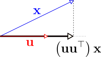
\[\mathbf{u}\mathbf{u}^\top=\begin{bmatrix} u_1^2 & u_1 u_2 & \cdots & u_1u_n \\ u_2u_1 & u_2^2 & \cdots & u_2u_n\\ \vdots & \vdots & \ddots & \vdots\\ u_nu_1 & u_n^2 & \cdots & u_n^2\end{bmatrix}\]This is the orthogonal projection matrix onto the space spanned by \(\mathbf{u}\), as shown in the following figure. The outer product appears in places involving orthogonal projections.
What if we wanted to do an orthogonal projection onto a subspace \(\mathcal{S}\) spanned by a set of vectors \(\left\{ \mathbf{x}_1, \mathbf{x}_2, \ldots \mathbf{x}_k \right\}\) that also form an orthonormal basis for \(\mathcal{S}\)?
We simply form a matrix \(\mathbf{X} = \begin{bmatrix} \mathbf{x}_1 & \mathbf{x}_2 & \cdots & \mathbf{x}_k \end{bmatrix}\) and the orthogonal projection matrix onto \(\mathcal{S}\) is given by,
\[\mathbf{P}_{\mathcal{S}}=\mathbf{X}\mathbf{X}^\top=\sum_{i=1}^k \mathbf{x}_i\mathbf{x}_i^\top \tag{2}\]When the basis \(\left\{ \mathbf{x}_1, \mathbf{x}_2, \ldots \mathbf{x}_k \right\}\) of \(\mathcal{S}\) is not orthonormal, the orthogonal projection matrix onto \(\mathcal{S}\) is given by,
\[\mathbf{P}_{\mathcal{S}} = \mathbf{X}\left(\mathbf{X}^\top\mathbf{X}\right)^{-1}\mathbf{X}^\top \tag{3}\]This does appear to have the outer product form but there is the strange inverse matrix in the middle. It can be shown that the product of three matrices \(\mathbf{A}\in\mathbb{R}^{n_1\times n_2}, \mathbf{B}\in\mathbb{R}^{n_2\times n_3}, \mathbf{C}\in\mathbb{R}^{n_3\times n_4}\) can be expressed as the following,
\[\mathbf{ABC} = \sum_{i=1}^{n_2}\sum_{j=1}^{n_3} b_{ij}\cdot \mathbf{a}_i\tilde{\mathbf{c}}_j^\top \tag{4}\]where,
- \(\mathbf{a}_i\) are the columns of \(\mathbf{A}\).
- \(\tilde{\mathbf{c}}_j^\top\) are the rows of \(\mathbf{C}\), and
- \(b_{ij}\) is the element in the \(i^{th}\) row and \(j^{th}\) column of \(\mathbf{B}\).
The product of these three matrices is the weighted linear combination of the outer product of the columns \(\mathbf{A}\) and the rows of \(\mathbf{C}\).
Let \(\mathbf{B}=\left(\mathbf{X}^\top\mathbf{X}\right)^{-1}\), then we have
\[\mathbf{P}_{\mathcal{S}}=\mathbf{X}\left(\mathbf{X}^\top\mathbf{X}\right)^{-1}\mathbf{X}^\top=\sum_{i=1}^{k}\sum_{j=1}^{k} b_{ij} \mathbf{x}_i\mathbf{x}_j^\top \tag{5}\]We again see that outer products come into the picture when dealing with orthogonal projection. Here, all possible \(k^2\) outer products are considered when the basis is not orthonormal. Equation (2) is a special case of Equation (5); when the basis is orthonormal the matrix \(\mathbf{X}^\top\mathbf{X}=\mathbf{I}_k\), which leaves only the outer products of the form \(\mathbf{x}_i\mathbf{x}_i^\top\).
We can think of the outer product \(\mathbf{u}\mathbf{v}^\top\) as a generalization of the orthogonal projection that we get with \(\mathbf{v}\mathbf{v}^\top\). I found a beautiful answer on StackOverflow about this here.
Consider three vectors, \(\mathbf{u}, \mathbf{v}, \mathbf{x} \in \mathbb{R}^n\), where \(\Vert \mathbf{u} \Vert = \Vert \mathbf{v} \Vert = 1\), then
\[\left(\mathbf{u}\mathbf{v}^\top\right)\mathbf{x} = \left(\mathbf{v}^\top \mathbf{x}\right)\mathbf{u}\]The outer product \(\mathbf{u}\mathbf{v}^\top\) is a matrix that help compute the component of \(\mathbf{x}\) along the \(\mathbf{v}\) direction taken along the \(\mathbf{u}\) direction. When \(\mathbf{u} = \mathbf{v}\), then this corresponds to the orthogonal projection operation, i.e. the component of \(\mathbf{x}\) along \(\mathbf{u}\), taken along \(\mathbf{u}\). This is demonstrated in the following figure.

The process of computing the components along one set of vectors and taking those components along another set of vectors is done by linear transformation represented by a matrix \(\mathbf{A}\).
Consider any matrix \(\mathbf{A} \in \mathbb{R}^{n \times m}\) of rank \(k\), which can be thought of as a linear transformation from \(\mathbb{R}^m\) to \(\mathbb{R}^n\). We can express this matrix using the SVD as the following,
\[\mathbf{A}=\mathbf{U}\mathbf{\Sigma}\mathbf{V}^\top, \quad \mathbf{U}\in\mathbb{R}^{n \times k}, \,\, \mathbf{V} \in \mathbb{R}^{m \times k}, \mathbf{\Sigma} \in \mathbb{R}^{k \times k}\] \[\mathbf{A}=\sum_{i=1}^k\sigma_i\mathbf{u}_i\mathbf{v }_i^\top\]The columns of \(\mathbf{V}\) form an orthonormal basis for the row space of \(\mathbf{A}\) and the columns of \(\mathbf{U}\) form an orthonormal basis of the column space of \(\mathbf{A}\). We could view the linear transformation performed by \(\mathbf{A}\) on a vector \(\mathbf{x}\in \mathbb{R}^m\) as the following,
- Find the components of the vector \(\mathbf{x}\) onto the right singular vectors \(\left\{\mathbf{v}_i\right\}_{i=1}^m\).
- Scale the individual components by the singular values \(\left\{\sigma_i\right\}_{i=1}^k\) .
- Compute the components along the left singular vectors \(\left\{\mathbf{u}_i\right\}_{i=1}^k\) using the scaling factor \(\left\{\sigma_i\mathbf{v}_i^\top\mathbf{x}\right\}_{i=1}^k\).
- Add these components to compute \(\mathbf{Ax}\).
In fact, we can think of the linear transformation performed by an matrix \(\mathbf{A}\) in a similar way when we can decompose the matrix as a product of two matrics, such as the LU decomposition,
\[\mathbf{A}=\mathbf{L}\mathbf{U}=\hat{\mathbf{L}}\mathbf{D}\hat{\mathbf{U}} = \sum_i d_i \mathbf{l}_i \tilde{\mathbf{u}}_i^\top\]- \(\mathbf{l}_i\) are the columns of \(\hat{\mathbf{L}}\) that form a basis for the column space of \(\mathbf{A}\), with unit length.
- \(\tilde{\mathbf{u}}_i^\top\) are the rows of \(\hat{\mathbf{U}}\) that form a basis for the row space of \(\mathbf{A}\), with unit length.
- \(\mathbf{D}\) is a diagonal matrix with the scaling factors.
The outer product is an fundamental operation in linear transformation. It allows us to represent and understand linear transformations as a superposition of simple transformations represented by rank-1 matrices.