\(\newcommand{\mf}{\mathbf} \newcommand{\mb}{\mathbb} \newcommand{\mc}{\mathcal}\) For full (column or row) rank non-square matrices \(\mf{A} \in \mb{R}^{n \times m}\), we can still have inverses but there are some peculiarities:
- We can only have left or right inverses, as is described below, and
- The left and right inverses are not unique.
We will talk about the inverses of tall matrices in this post, i.e. matrices where $n > m$. Tall full rank matrices only have left inverses:
\[n > m, \,\, rank\left(\mf{A}\right) = m \implies \exists \mf{B} \in \mb{R}^{m \times n} \,\, s.t. \,\, \mf{B} \mf{A} = \mf{I}_{m}\]This means that, $\mf{B}\mf{A}\mf{x} = \mf{B}\mf{y} \implies \mf{x} = \mf{B}\mf{y}$.
What $\mf{x}$ represents depends on whether or not $\mf{y}$ is in the column space of $\mf{A}$.
- $\mf{y} \in \mc{C}\left( \mf{A} \right) \implies $ $\mf{x} = \mf{B}\mf{y}$ is the representation of $\mf{y}$ in the column basis of $\mf{A}$.
- $\mf{y} \notin \mc{C}\left( \mf{A} \right) \implies $ $\mf{x} = \mf{Bb}$ is the representation of some vector $\hat{\mf{y}}$ $=$ $\mf{A}\mf{x} = \mf{ABb}$, which in the column basis of $\mf{A}$.
When $\mf{x}$ is substituted back into the original equation, we get
\[\begin{cases} \mf{y} \in \mc{C}\left(\mf{A}\right) &\implies \hat{\mf{y}} = \mf{A}\left(\mf{B}\mf{y}\right) = \mf{y} \\ \mf{y} \notin \mc{C}\left(\mf{A}\right) &\implies \hat{\mf{y}} = \mf{A}\left(\mf{B}\mf{y}\right) \neq \mf{y} \end{cases}\]For a given left inverse $\mf{B}$, adding a matrix $\mf{C}$ whose rows are orthogonal to the columns of $\mf{A}$ will result in another left inverse of $\mf{A}$.
\[\left( \mf{B} + \mf{C} \right) \mf{A} = \mf{I}_m, \, s.t. \, \mf{C}\mf{A} = \mf{0}\]The rows of $\mf{C}$ will be vectors from $\mc{N}\left(\mf{A}^\top\right)$ - the left nullspace of $\mf{A}$. Thus, it is clear that there are infinitely many left inverses for $\mf{A}$.
What do all these left inverse matrices do?
A left inverse allows us to find the representation of \(\hat{\mf{y}}\) – a component of \(\mf{y}\) in \(\mc{C}\left(\mf{A}\right)\) – in the column basis of \(\mf{A}\).
These components are oblique projections onto \(\mc{C}\left(\mf{A}\right)\) along a complementary subspace to \(\mc{C}\left(\mf{A}\right)\) in \(\mb{R}^n\). The matrix \(\mf{A}\left( \mf{B} + \mf{C}\right)\) is this oblique projection matrix.
\[\hat{\mf{y}} = \mf{A}\left(\mf{B} + \mf{C}\right) \mf{y}\]In the absence of a mathetical proof of this, let’s convince ourselves that this is true through a simple example. Let \(\mf{A} = \begin{bmatrix} 1 \\ 1\end{bmatrix}\). The following are the various possible left inverses of \(\mf{A}\),
\[\mf{B} + \mf{C} = \begin{bmatrix} \mf{\tilde{b}}_1^\top \end{bmatrix} + \begin{bmatrix} \mf{\tilde{c}}_1^\top \end{bmatrix} = \frac{1}{2}\begin{bmatrix} 1 & 1 \end{bmatrix} + \begin{bmatrix} \alpha & -\alpha \end{bmatrix}\]The following figures depicts this particular example,
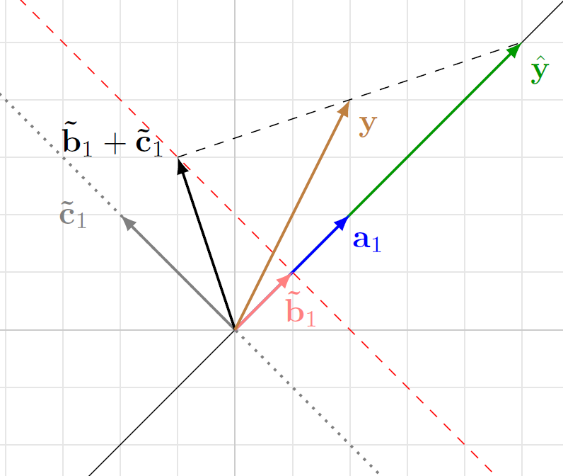
In this figure, we have assumed \(\alpha = -1 \implies \mf{\tilde{c}}_1 = \begin{bmatrix} -1 \\ 1\end{bmatrix}\), and \(\mf{y} = \begin{bmatrix} 1 \\ 2\end{bmatrix}\). Thus,
\[\begin{split} \hat{\mf{y}} &= \mf{A} \left( \mf{B} + \mf{C}\right) \mf{y} \\ &= \begin{bmatrix} 1 \\ 1\end{bmatrix} \begin{bmatrix} -\frac{1}{2} & \frac{3}{2}\end{bmatrix} \begin{bmatrix} 1 \\ 2\end{bmatrix} \\ &= \begin{bmatrix} \frac{5}{2} \\ \frac{5}{2} \end{bmatrix} \end{split}\]\(\hat{\mf{y}}\) is the oblique projection of \(\mf{y}\) onto \(\mc{C}\left(\mf{A}\right)\) along the subspace parallel to the dashed black line joining \(\mf{y}\) and \(\hat{\mf{y}}\) in the above figure. This is the subspace spanned by the vector \(\mf{y} - \hat{\mf{y}} = \begin{bmatrix} \frac{3}{2} \\ \frac{1}{2} \end{bmatrix}\). It is important to that \(\mf{\tilde{b}}_1 + \mf{\tilde{c}}_1\) is orthogonal to \(\mf{y} - \hat{\mf{y}}\).
\[\left( \mf{\tilde{b}}_1 + \mf{\tilde{c}}_1\right)^\top\left( \mf{y} - \hat{\mf{y}} \right) = 0\]The following examples demonstrates the same for a different value of \(\alpha = 2.5\).
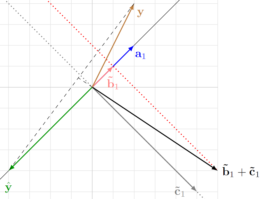
It is left as an exercise to work out the different components and verfiy that \(\left( \mf{\tilde{b}}_1 + \mf{\tilde{c}}_1\right) \perp \left(\mf{y} - \hat{\mf{y}}\right)\).
For any choice of \(\alpha\) we can get a oblique project matrix onto \(\mc{C}\left(\mf{A}\right)\) along a subspace orthogonal to that of \(\mc{C}\left(\mf{B}^\top + \mf{C}^\top\right)\), i.e. the row space of the left inverse.
A special left inverse.
Among the infintely many oblique projectors, the orthogonal projector is a speical one. The left inverse of \(\mf{A}\) that will allow us to do orthogonal projection is the Moore-Penrose Inverse or the Pseudoinverse, expressed as \(\mf{A}^\dagger\).
\[\mf{A}^\dagger = \left(\mf{A}^\top\mf{A}\right)^{-1}\mf{A}^\top\]The matrix \(\mf{B} = \begin{bmatrix} \mf{\tilde{b}}_1^\top \end{bmatrix} = \frac{1}{2}\begin{bmatrix} 1 & 1 \end{bmatrix}\) shown in the above figures is the pseudoinverse of \(\mf{A}\).
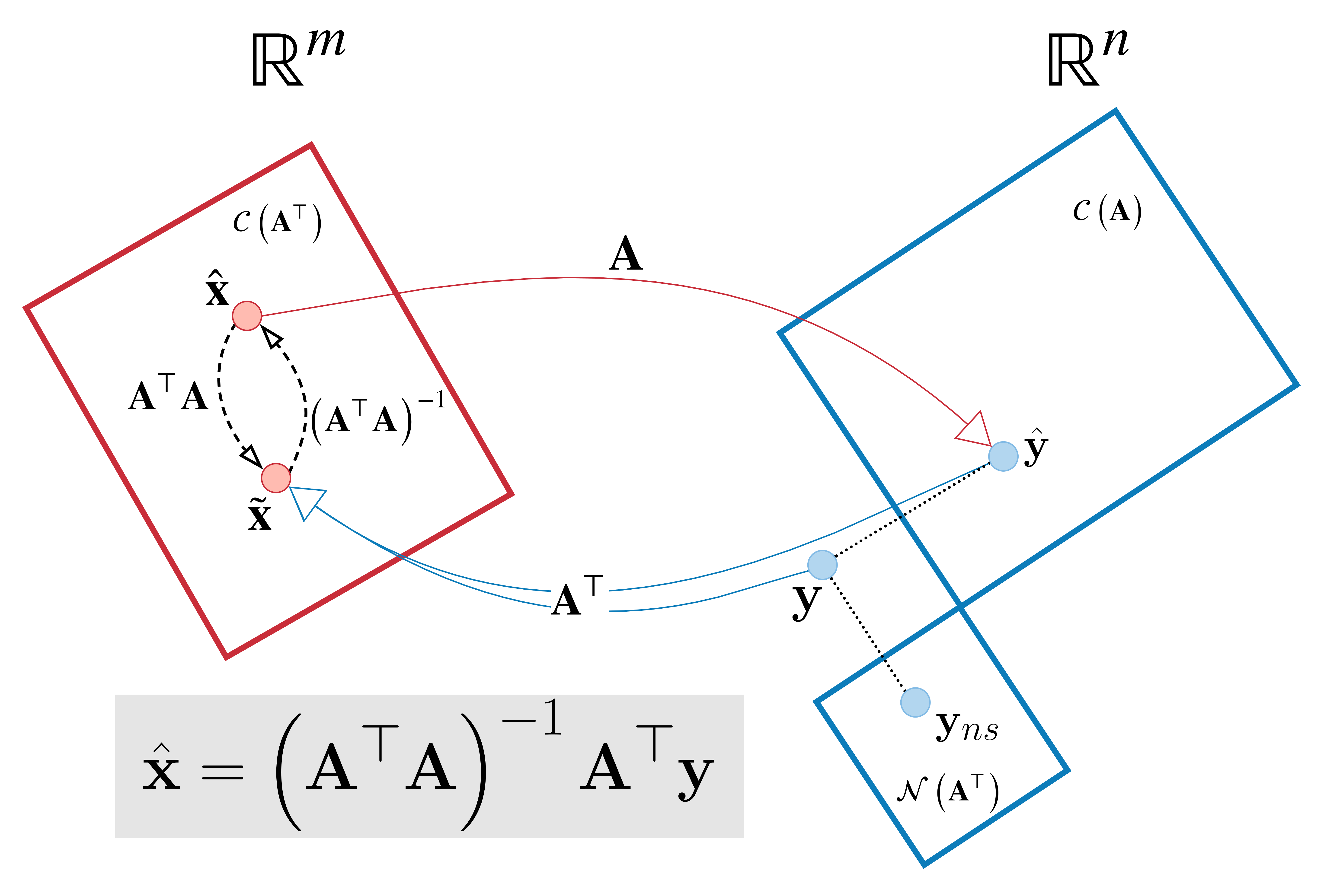
The mapping performed by the psuedoinverse \(\mathbf{A}^\dagger\) is shown in the above figure.
How do know that this is in fact a orthogonal projector?
\(\mc{C}\left(\left(\mf{A}^\dagger\right)^\top\right) = \mc{C}\left(\mf{A}\right)\), which means that the matrix \(\mf{A}\mf{A}^\dagger\) is the projection matrix onto \(\mc{C}\left( \mf{A} \right)\) along the subspace orthogonal to \(\mc{C}\left(\mf{A}\right)\), which is \(\mc{N}\left(\mf{A}^\top\right)\).
I hope this short presentaion helps shed some light on the geometry operation behind left inverses. The next part of this series will focus on the right inverse.