Matrices are a representation of linear maps between finite-dimensional vector spaces. Consider a linear map \(\mathcal{L}\) from \(\mathbb{R}^m\) to \(\mathbb{R}^n\).
\[\mathcal{L}: \mathbb{R}^m \mapsto \mathbb{R}^n\]This linear map can be represented using a real matrix \(\mathbf{A} \in \mathbb{R}^{n \times m}\), such that
\[\mathbf{y} = \mathcal{L}\left( \mathbf{x} \right) = \mathbf{A}\mathbf{x}, \quad \mathbf{x} \in \mathbb{R}^m, \, \mathbf{y} \in \mathbb{R}^n\]When the domain and range spaces are the same, then \(\mathbf{A}\) is a square matrix.
The matrix \(\mathbf{A}\) has a unique inverse \(\mathbf{A}^{-1}\), if and only if the \(\mathbf{A}\) is full-rank, i.e. the columns of the matrix form a basis for \(\mathbb{R}^n\). In this case, \(\mathbf{A}^{-1}\mathbf{A} = \mathbf{A}\mathbf{A}^{-1} = \mathbf{I}_n\), where \(\mathbf{I}_n\) is the \(n \times n\) identity matrix.
Matrix inverses allow us to change basis
Consider the equation, \(\mathbf{A}\mathbf{x} = \mathbf{y}\). This equation says that the vector \(\mathbf{y}\) is a linear combination of the columns of \(\mathbf{A}\), with the weight for each column given by the elements of \(\mathbf{x}\).
\[\mathbf{y} = \mathbf{A}\mathbf{x} = \begin{bmatrix} \mathbf{a}_1 & \mathbf{a}_2 & \cdots & \mathbf{a}_n\end{bmatrix} \begin{bmatrix} x_1 \\ x_2 \\ \vdots \\ x_n\end{bmatrix} = \sum_{i=1}^n x_i\mathbf{a}_i\]Here, \(\mathbf{x}\) is the representation of the vector \(\mathbf{y}\) in the basis of \(\mathbb{R}^n\) formed by the columns of \(\mathbf{A}\) (we will refer to this basis as the column basis). Given \(\mathbf{A}\) and \(\mathbf{y}\), we can solve for \(\mathbf{x}\) using the inverse of \(\mathbf{A}\),
\[\mathbf{x} = \mathbf{A}^{-1}\mathbf{y}\]Thus, we see that \(\mathbf{A}^{-1}\) is the matrix that allows us to change the representation of a vector to the column basis.
Structure of a matrix inverse Let us express $\mathbf{A}^{-1}$ as a column of rows.
\[\mathbf{A} = \begin{bmatrix} \mathbf{a}_1 & \mathbf{a}_2 & \ldots & \mathbf{a}_n \end{bmatrix} \longrightarrow \mathbf{A}^{-1} = \begin{bmatrix} \mathbf{\tilde{b}}_1^\top \\ \mathbf{\tilde{b}}_2^\top \\ \vdots \\ \mathbf{\tilde{b}}_n^\top\end{bmatrix}\]Let \(\mathbf{A} = \begin{bmatrix} 1 & 1\\ 0 & 1 \end{bmatrix} = \begin{bmatrix} \mathbf{a}_1 & \mathbf{a}_2 \end{bmatrix}\), then \(\mathbf{A}^{-1} = \begin{bmatrix} 1 & -1 \\ 0 & 1\end{bmatrix} = \begin{bmatrix} \mathbf{\tilde{b}_1^\top} \\ \mathbf{\tilde{b}_2^\top}\end{bmatrix}\). Here,
\[\mathbf{\tilde{b}}_1^\top \mathbf{a}_1 = \mathbf{\tilde{b}}_2^\top \mathbf{a}_2 = 1 \quad \text{and} \quad \mathbf{\tilde{b}}_1^\top \mathbf{a}_2 = \mathbf{\tilde{b}}_2^\top \mathbf{a}_1 = 0\]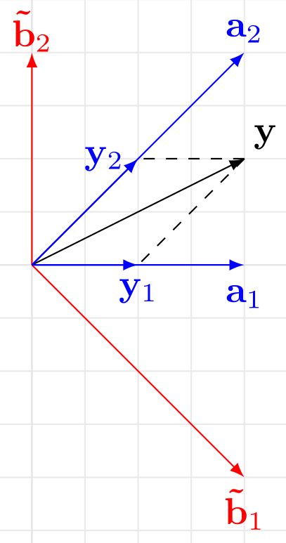
The components of $\mathbf{y}$ in column basis is given by, \(\mathbf{x} = \begin{bmatrix} x_1 \\ x_2 \end{bmatrix} = \mathbf{A}^{-1}\mathbf{y}\).
\[x_1 = \mathbf{\tilde{b}}_1^\top \mathbf{y} \quad \quad x_2 = \mathbf{\tilde{b}}_2^\top \mathbf{y}\]Here, $\mathbf{y}_1 = x_1 \mathbf{y}$ is the oblique projection of $\mathbf{y}$ onto the subspace spanned by $\mathbf{a}_1$, along the subspace spanned by $\mathbf{a}_2$. The scaling factor $x_1$ for this oblique projection is obtained by taking the inner product of $\mathbf{y}$ with $\mathbf{\tilde{b}}_1$.
Similarly, $\mathbf{y}_2 = x_2 \mathbf{a}_2$ is the oblique projection of $\mathbf{y}$ onto the subspace spanned by $\mathbf{a}_2$ along the subspace spanned by $\mathbf{a}_1$. $x_2$ is obtained by taking the inner product of $\mathbf{y}$ with $\mathbf{\tilde{b}}_2$.
This can be generalized to a $n \times n$ square matrix $\mathbf{A}$.
The oblique projection of $\mathbf{y}$ onto \(span\left( \{ \mathbf{a}_i \}\right)\) along \(span\left( \{ \mathbf{a}_j \}_{j=1, j \neq i}^{n}\right)\) is obtained by computing the scaling factor $x_i$ as the following,
\[x_i = \mathbf{\tilde{b}}_i^\top \mathbf{y}\] \[\mathbf{y}_i = x_i \mathbf{a}_i = \left( \mathbf{\tilde{b}}_i^\top \mathbf{y} \right) \mathbf{a}_i = \left( \mathbf{a}_i \mathbf{\tilde{b}}_i^\top \right) \mathbf{y} = \mathbf{P}_i \mathbf{y}\]Note: \(span\left( \{ \mathbf{a}_j \}_{j=1, j \neq i}^{n}\right)\) is the subspace spanned by the columns of \(\mathbf{A}\) except \(\mathbf{a}_i\).
\(\mathbf{P}_i = \mathbf{a}_i \mathbf{\tilde{b}}_i^\top\) is the projection matrix that does oblique projections onto \(span\left( \{ \mathbf{a}_i \}\right)\) along \(span\left( \{ \mathbf{a}_j \}_{j=1, j \neq i}^{n}\right)\).
\[\mathbf{x} = \begin{bmatrix} x_1 \\ x_2 \\ \vdots \\ x_n \end{bmatrix} = \mathbf{A}^{-1} \mathbf{y} = \begin{bmatrix} \mathbf{\tilde{b}}_1^\top \\ \mathbf{\tilde{b}}_2^\top \\ \vdots \\ \mathbf{\tilde{b}}_n^\top \end{bmatrix} \mathbf{y} = \begin{bmatrix} \mathbf{\tilde{b}}_1^\top \mathbf{y} \\ \mathbf{\tilde{b}}_2^\top \mathbf{y} \\ \vdots \\ \mathbf{\tilde{b}}_n^\top \mathbf{y} \end{bmatrix}\]The matrix \(\mathbf{P}_{1:r} = \sum_{i=1}^{r} \mathbf{P}_i = \sum_{i=1}^{r} \mathbf{a}_i \mathbf{\tilde{b}}_i^\top\) is the oblique projection matrix onto \(span\left( \{ \mathbf{a}_i \}_{i=1}^{r}\right)\) along \(span\left( \{ \mathbf{a}_i \}_{i=r+1}^{n}\right)\).
Taking the inner product with the rows \(\left\{ \mathbf{\tilde{b}}_i^\top \right\}_{i=1}^r\) will give us the scaling factors required to obtain the oblique projection along the subspace that is orthogonal to \(span\left( \left\{ \mathbf{\tilde{b}}_i \right\}_{i=1}^r \right)\), which is \(span\left( \left\{ \mathbf{a}_i \right\}_{i=r+1}^n\right)\). This fact will come in handy in understanding the geometric operations performed by left inverses.
In the next two parts of the blog on matrix inverses, we will go into the details of left and right inverses of full rank rectangular matrices.